{
"cells": [
{
"cell_type": "markdown",
"metadata": {
"collapsed": true
},
"source": [
"# *Chapter 11*
Applied HPC: Optimization, Tuning & GPU Programming \n",
"\n",
"| | | |\n",
"|:---:|:---:|:---:|\n",
"| |[From **COMPUTATIONAL PHYSICS**, 3rd Ed, 2015](http://physics.oregonstate.edu/~rubin/Books/CPbook/index.html)
RH Landau, MJ Paez, and CC Bordeianu (deceased)
Copyrights:
[Wiley-VCH, Berlin;](http://www.wiley-vch.de/publish/en/books/ISBN3-527-41315-4/) and [Wiley & Sons, New York](http://www.wiley.com/WileyCDA/WileyTitle/productCd-3527413154.html)
R Landau, Oregon State Unv,
MJ Paez, Univ Antioquia,
C Bordeianu, Univ Bucharest, 2015.
Support by National Science Foundation.|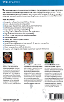|\n",
"\n",
"> More computing sins are committed in the name of efficiency (without necessarily achieving it) than for any other single reason - including blind stupidity. - W.A. Wulf\n",
">\n",
"> We should forget about small efficiencies, say about 97% of the time:
\n",
"> premature optimization is the root of all evil. - Donald Knuth\n",
">\n",
"> The best is the enemy of the good. - Voltaire\n",
"\n",
"**11 Applied HPC: Optimization, Tuning & GPU Programming**
\n",
"[11.1 General Program Optimization](#11.1)
\n",
" [11.1.1 Programming for Virtual Memory](#11.1)
\n",
" [11.1.2 Optimization Exercises](#11.1)
\n",
"[11.2 Optimized Matrix Programming with NumPy](#11.1)
\n",
" 11.2.1 NumPy Optimization Exercises](#11.1)
\n",
"[11.3 Empirical Performance of Hardware](#11.1)
\n",
" 11.3.1 Racing Python versus Fortran/C](#11.1)
\n",
"[11.4 Programming for the Data Cache (Method)](#11.1)
\n",
" [11.4.1 Exercise 1: Cache Misses](#11.1)
\n",
" [11.4.2 Exercise 2: Cache Flow](#11.1)
\n",
" [11.4.3 Exercise 3: Large-Matrix Multiplication](#11.1)
\n",
"[11.5 Graphical Processing Units for High Performance Computing](#11.1)
\n",
" 11.5.1 The GPU Card](#11.1)
\n",
"[11.6 Practical Tips for Multicore & GPU Programming](#11.1)
\n",
" [11.6.1 CUDA Memory Usage](#11.1)
\n",
" [11.6.2 CUDA Programming](#11.1)
\n",
"\n",
"*This chapter continues the discussion of high-performance computing\n",
"(HPC) began in the previous chapter. Here we lead the reader through\n",
"exercises that demonstrates some techniques for writing programs that\n",
"are optimized for HPC hardware, and how the effects of optimization may\n",
"be different in different computer languages. We then move on to tips\n",
"for programming on a multicore computer. We conclude with an example of\n",
"programming in Compute Unified Device Architecture (CUDA) on a graphics\n",
"processing card, a subject beyond the general scope of this text, but\n",
"one of high current interest.*\n",
"\n",
"[All Lectures ](http://physics.oregonstate.edu/~rubin/Books/CPbook/eBook/Lectures/index.html)\n"
]
},
{
"cell_type": "markdown",
"metadata": {},
"source": [
"## 11.1 General Program Optimization\n",
"\n",
"*Rule 1: Do not do it.*\n",
"\n",
"*Rule 2 (for experts only): Do not do it yet.*\n",
"\n",
"*Rule 3: Do not optimize as you go: Write your program without regard to\n",
"possible optimizations, concentrating instead on making sure that the\n",
"code is clean, correct, and understandable. If it’s too big or too slow\n",
"when you’ve finished, then you can consider optimizing it.*\n",
"\n",
"*Rule 4: Remember the 80/20 rule: In many fields you can get 80% of the\n",
"result with 20% of the effort (also called the 90/10 rule - it depends\n",
"on who you talk to). Whenever you’re about to optimize code, use\n",
"profiling to find out where that 80% of execution time is going, so you\n",
"know where to concentrate your effort.*\n",
"\n",
"*Rule 5: Always run “before” and “after” benchmarks: How else will you\n",
"know that your optimizations actually made a difference? If your\n",
"optimized code turns out to be only slightly faster or smaller than the\n",
"original version, undo your changes and go back to the original, clear\n",
"code.*\n",
"\n",
"*Rule 6: Use the right algorithms and data structures: Do not use an\n",
"$\\mathcal{O}(n^2)$ DFT algorithm to do a Fourier transform of a thousand\n",
"elements when there’s an $\\mathcal{O}(n \\log n)$ FFT available.\n",
"Similarly, do not store a thousand items in an array that requires an\n",
"$\\mathcal{O}(n)$ search when you could use an $\\mathcal{O}(\\log n)$\n",
"binary tree or an $\\mathcal{O}(1)$ hash table.* \\[[Hardwich(96))](BiblioLinked.html#Har96)\\]\n",
"\n",
"The type of optimization often associated with *high-performance* or\n",
"*numerically intensive* computing is one in which sections of a program\n",
"are rewritten and reorganized in order to increase the program’s speed.\n",
"The overall value of doing this, especially as computers have become so\n",
"fast and so available, is often a subject of controversy between\n",
"computer scientists and computational scientists. Both camps agree that\n",
"using the optimization options of compilers is a good idea. Yet on the\n",
"one hand, CS tends to think that optimization is best left to the\n",
"compilers, while computational scientists, who tend to run large codes\n",
"with large amounts of data in order to solve real-world problems, often\n",
"believe that you cannot rely on the compiler to do all the optimization.\n",
"\n",
"### 11.1.1 Programming for Virtual Memory (Method)\n",
"\n",
"While memory paging makes little appear big, you pay a price because\n",
"your program’s run time increases with each page fault. If your program\n",
"does not fit into RAM all at once, it will be slowed down significantly.\n",
"If virtual memory is shared among multiple programs that run\n",
"simultaneously, they all can’t have the entire RAM at once, and so there\n",
"will be memory access *conflicts* which will decrease performance. The\n",
"basic rules for programming for virtual memory are:\n",
"\n",
"1. Do not waste your time worrying about reducing the amount of memory\n",
" used (the *working set size*) unless your program is large. In that\n",
" case, take a global view of your entire program and optimize those\n",
" parts that contain the largest arrays.\n",
"\n",
"2. Avoid page faults by organizing your programs to successively\n",
" perform their calculations on subsets of data, each fitting\n",
" completely into RAM.\n",
"\n",
"3. Avoid simultaneous calculations in the same program to avoid\n",
" competition for memory and consequent page faults. Complete each\n",
" major calculation before starting another.\n",
"\n",
"4. Group data elements close together in memory blocks if they are\n",
" going to be used together in calculations."
]
},
{
"cell_type": "markdown",
"metadata": {},
"source": [
"### 11.1.2 Optimization Exercises\n",
"\n",
"Many of the optimization techniques developed for Fortran and C are also\n",
"relevant for Python applications. Yet while Python is a good language\n",
"for scientific programming and is as universal and portable as Java, at\n",
"present Python code runs slower than Fortran, C or even Java codes. In\n",
"part, this is a consequence of the Fortran and C compilers having been\n",
"around longer and thereby having been better refined to get the most out\n",
"of a computer’s hardware, and in part this is also a consequence of\n",
"Python not being designed for speed. Because modern computers are so\n",
"fast, whether a program takes 1s or 3s usually does not matter much,\n",
"especially in comparison to the hours or days of *your* time that it\n",
"might take to modify a program for increased speed. However, you may\n",
"want to convert the code to C (whose command structure is similar to\n",
"that of Python) if you are running a computation that takes hours or\n",
"days to complete and will be doing it many times.\n",
"\n",
"Especially when asked to, compilers may look at your entire code as a\n",
"single entity and rewrite it in an attempt to make it run faster. In\n",
"particular, Fortran and C compilers often speed up programs by being\n",
"careful in how they load arrays into memory. They also are careful in\n",
"keeping the cache lines full so as not to keep the CPU waiting or having\n",
"it move on to some other chore. That being said, in our experience\n",
"compilers still cannot optimize a program as well as can a skilled and\n",
"careful programmer who understands the order and structure of the code.\n",
"\n",
"There is no fundamental reason why a program written in Java or Python\n",
"cannot be compiled to produce a highly efficient code, and indeed such\n",
"compilers are being developed and becoming available. However, such code\n",
"is optimized for a particular computer architecture and so is not\n",
"portable. In contrast, the byte code ( `.class` file in Java and `.pyc`\n",
"file in Python) produced by the compiler is designed to be interpreted\n",
"or recompiled by theJava or Python *Virtual Machine* (just another\n",
"program). When you change from Unix to Windows, for example, the Virtual\n",
"Machine program changes, but the byte code is the same. This is the\n",
"essence of portability.\n",
"\n",
"In order to improve the performance of Java and Python, many computers\n",
"and browsers run *Just-in-Time* (JIT) compilers. If a JIT is present,\n",
"the Virtual Machine feeds your byte code `Prog.class` or ` Prog.pyc` to\n",
"the JIT so that it can be recompiled into native code explicitly\n",
"tailored to the machine you are using. Although there is an extra step\n",
"involved here, the total time it takes to run your program is usually\n",
"10-30 times faster with a JIT as compared to line-by-line\n",
"interpretation. Because the JIT is an integral part of the Virtual\n",
"Machine on each operating system, this usually happens automatically.\n",
"\n",
"In the experiments below you will investigate techniques to optimize\n",
"both Fortran and Java or Python programs, and to compare the speeds of\n",
"both languages for the same computation. If you run your program on a\n",
"variety of machines you should also be able to compare the speed of one\n",
"computer to that of another. Note that a knowledge of Fortran or C is\n",
"not required for these exercises; if you keep an open mind you should be\n",
"able to look at the code and figure out what changes may be needed.\n",
"\n",
"#### Good and Bad Virtual Memory Use (Experiment)\n",
"\n",
"To see the effect of using virtual memory, convert these simple\n",
"pseudocode examples (Listings 11.1 and 11.2) into actual code in your\n",
"favorite language, and then run them on your computer. Use a command\n",
"such as `time, time.clock()` or `timeit` to measure the time used for\n",
"each example. These examples call functions `force12` and `force21`. You\n",
"should write these functions and make them have significant memory\n",
"requirements.\n",
"\n",
"**Listing 11.1 BAD program, too simultaneous.**\n",
"\n",
" for j = 1, n; { for i = 1, n; {\n",
" f12(i,j) = force12(pion(i), pion(j)) // Fill f12\n",
" f21(i,j) = force21(pion(i), pion(j)) // Fill f21\n",
" ftot = f12(i,j) + f21(i,j) } } // Fill ftot\n",
"\n",
"You see (Listing 11.1) that each iteration of the `for` loop requires\n",
"the data and code for all the functions as well as access to all the\n",
"elements of the matrices and arrays. The working set size of this\n",
"calculation is the sum of the sizes of the arrays `f12(N,N)`,\n",
"`f21(N,N)`, and `pion(N)` plus the sums of the sizes of the functions\n",
"`force12` and `force21`.\n",
"\n",
"A better way to perform the same calculation is to break it into\n",
"separate components (Listing 11.2):\n",
"\n",
"**Listing 12.2 GOOD program, separate loops.**\n",
"\n",
" for j = 1, n;\n",
" { for i = 1, n; f12(i,j) = force12(pion(i), pion(j)) }\n",
" for j = 1, n;\n",
" { for i = 1, n; f21(i,j) = force21(pion(i), pion(j)) }\n",
" for j = 1, n;\n",
" { for i = 1, n; ftot = f12(i,j) + f21(i,j) }\n",
"\n",
"Here the separate calculations are independent and the *working set\n",
"size*, that is, the amount of memory used, is reduced. However, you do\n",
"pay the additional overhead costs associated with creating extra `for`\n",
"loops. Because the working set size of the first `for` loop is the sum\n",
"of the sizes of the arrays `f12(N, N)` and `pion(N)`, and of the\n",
"function `force12`, we have approximately half the previous size. The\n",
"size of the last `for` loop is the sum of the sizes for the two arrays.\n",
"The working set size of the entire program is the larger of the working\n",
"set sizes for the different `for` loops.\n",
"\n",
"As an example of the need to group data elements close together in\n",
"memory or common blocks if they are going to be used together in\n",
"calculations, consider the following code (Listing 11.3):\n",
"\n",
"**Listing 11.3 BAD Program, discontinuous memory.**\n",
"\n",
" Common zed, ylt(9), part(9), zpart1(50000), zpart2(50000), med2(9)\n",
" for j = 1, n;\n",
" ylt(j) = zed * part(j)/med2(9) // Discontinuous variables\n",
"\n",
"Here the variables `zed`, `ylt`, and `part` are used in the same\n",
"calculations and are adjacent in memory because the programmer grouped\n",
"them together in `Common` (global variables). Later, when the programmer\n",
"realized that the array `med2` was needed, it was tacked onto the end of\n",
"`Common`. All the data comprising the variables `zed`, `ylt`, and `part`\n",
"fit onto one page, but the `med2` variable is on a different page\n",
"because the large array `zpart2(50000)` separates it from the other\n",
"variables. In fact, the system may be forced to make the entire 4-kB\n",
"page available in order to fetch the 72 B of data in `med2`. While it is\n",
"difficult for a Fortran or C programmer to establish the placement of\n",
"variables within page boundaries, you will improve your chances by\n",
"grouping data elements together (Listing 11.4):\n",
"\n",
"**Listing 11.4 GOOD program, continuous memory.**\n",
"\n",
" Common zed, ylt(9), part(9), med2(9), zpart1(50000), zpart2(50000)\n",
" for j = 1, n;\n",
" ylt(j) = zed*part(j)/med2(J) // Continuous"
]
},
{
"cell_type": "markdown",
"metadata": {},
"source": [
"## 11.2 Optimized Matrix Programming with NumPy\n",
"\n",
"In [Chapter 6](CP06.ipynb) we demonstrated several ways of handling\n",
"matrices with Python. In particular, we recommended using the `array`\n",
"structure and the NumPy package. In this section we extend that\n",
"discussion somewhat by demonstrating two ways in which NumPy may speed\n",
"up a program. The first is by using NumPy arrays rather than Python\n",
"ones, and the second is by using Python slicing to reduce stride.\n",
"\n",
"[**Listing 11.5 TuneNumPy.py**](http://www.science.oregonstate.edu/~rubin/Books/CPbook/Codes/HPCodes/TuneNumpy.py) compares the time it takes to evaluate a\n",
"function of each element of an array using a for loop, as well as using a\n",
"vectorized call with NumPy. To see the effect of fluctuations, the comparison is\n",
"repeated three times.\n",
"\n",
"A powerful feature of NumPy is its high-level *vectorization*. This is\n",
"the process in which the single call of a function operates not on a\n",
"variable but on an array object as a whole. In the latter case, NumPy\n",
"automatically *broadcasts* the operation across all elements of the\n",
"array with efficient use of memory. As we shall see, the resulting speed\n",
"up can be more than an order of magnitude! While this may sound\n",
"complicated, it really is quite simple because NumPy does this for you\n",
"automatically.\n",
"\n",
"For example, in Listing 11.5 we present the code `TuneNumpy.py`. It\n",
"compares the speed of a calculation using a *for* loop to evaluate a\n",
"function for each of 100,000 elements in an array, versus the speed\n",
"using NumPy’s vectorized evaluation of that function for an array object\n",
"\\[[CiSE(15))](BiblioLinked.html#CiSE)\\]. And to see the effects of fluctuations as a result of\n",
"things like background processes, we repeat the comparison three times.\n",
"We obtained the results:\n",
"\n",
" For for loop, t2-t1 = 0:00:00.384000\n",
" For vector function, t2-t1 = 0:00:00.009000\n",
" For for loop, t2-t1 = 0:00:00.383000\n",
" For vector function, t2-t1 = 0:00:00.009000\n",
" For for loop, t2-t1 = 0:00:00.387000\n",
" For vector function, t2-t1 = 0:00:00.008000\n",
"\n",
"\n",
"Though a simple calculation, these results show that vectorization\n",
"speeds the calculation up by a factor of nearly 50; really!\n",
"\n",
"Now recall from earlier in this chapter our discussion of *stride* (the\n",
"amount of memory skipped in order to get to the next element needed in a\n",
"calculation). It is important to have your program minimize stride in\n",
"order not waste time jumping through memory, as well as not to load\n",
"unneeded data into memory. For example, for a (1000, 1000) array, there\n",
"is a passage of 1 word to get to the next column, but of 1000 words to\n",
"get to the next row. Clearly better to do a column-by-column calculation\n",
"than a row-by-row one.\n",
"\n",
"We start our example by setting up a $3\\times 3$ array of integers using\n",
"NumPy’s `arange` to create a 1D array. We then reshape it into a\n",
"$3\\times3$ array and determine the strides of the matrix for rows and\n",
"columns:\n",
"\n",
" >>> from numpy import *\n",
" >>> A = arange(0,90,10)\n",
" >>> A\n",
" array([ 0, 10, 20, 30, 40, 50, 60, 70, 80])\n",
" >>> A = A.reshape((3,3))\n",
" >>> A\n",
" array([[ 0, 10, 20],\n",
" [30, 40, 50],\n",
" [60, 70, 80]])\n",
" >>> A.strides\n",
" (12, 4)\n",
"\n",
"Line 11 tells us that it takes 12 bytes (3 values) to get to the same\n",
"position in the next row, but only 4 bytes (one value) to get to the\n",
"same position in the next column. Clearly cheaper to go from column to\n",
"column. Now we show you an easy way to do that.\n",
"\n",
"Recall Python’s *slice* operator that extracts just the desired part of\n",
"a list (like taking a “slice” through the center of a jelly doughnut):\n",
"`ListName[StartIndex:StopBeforeIndex:Step]`.\n",
"The convention here is that if no argument is given, then the slice\n",
"starts at 0 and stops at the end of the list. For example:\n",
"\n",
" >>> A = arange(0,90,10).reshape((3,3))\n",
" >>> A\n",
" array([[ 0, 10, 20],\n",
" [30, 40, 50],\n",
" [60, 70, 80]])\n",
" >>> A[:2,:] # First two rows (start at 2, go to end)\n",
" array([[ 0, 10, 20],\n",
" [30, 40, 50]])\n",
" >>> A[:,1:3] # Columns 1-3 (start at 1, end at 4)\n",
" array([[10, 20],\n",
" [40, 50],\n",
" [70, 80]])\n",
" >>> A[::2,:] # Every second row\n",
" array([[ 0, 10, 20],\n",
" [60, 70, 80]])\n",
"\n",
"Once sliced, Python does not have to jump through memory to work with\n",
"these elements, or even set up separate arrays for them. This is called\n",
"*view-based indexing*, with the indexed notation returning a new array\n",
"object that *points* to the address of the original data rather than\n",
"store the values of the new array (think “pointers” in C). This does\n",
"lead to improved speed, but you must remember that if you alter the new\n",
"array, you are also altering the original array to which it points\n",
"(think “pointers” in C).\n",
"\n",
"For instance, you can optimize a finite difference calculation of\n",
"forward and central difference derivatives quite elegantly \\[CiSE(15)\\]:\n",
"\n",
" >>> x = arange(0,20,2)\n",
" >>> x\n",
" array([ 0, 2, 4, 6, 8, 10, 12, 14, 16, 18])\n",
" >>> y = x**2\n",
" >>> y\n",
" array([ 0, 4, 16, 36, 64, 100, 144, 196, 256, 324], dtype=int32)\n",
" >>> dy_dx = ((y[1:]-y[:1])/(x[1:]-x[:-1])) # Forward difference\n",
" >>> dy_dx\n",
" array([ 2., 8., 18., 32., 50., 72., 98., 128., 162.])\n",
" >>> dy_dx_c = ((y[2:]-y[:-2])/(x[2:]-x[:-2])) # Central difference\n",
" >>> dy_dx_c\n",
" array([ 4., 8., 12., 16., 20., 24., 28., 32.])\n",
"\n",
"(We note that the values of the derivatives look quite different, yet\n",
"the forward difference is evaluated at the start of the interval and the\n",
"central difference at the center.)\n",
"\n",
"### 11.2.1 NumPy Optimization Exercises\n",
"\n",
"1. We have just demonstrated how NumPy’s vectorized function evaluation\n",
" can speed up a calculation by a factor of 50 via via broadcast of an\n",
" operation over an array rather than performing that operation on\n",
" each individual element in the array. Determine the speedup for the\n",
" matrix multiplication $[A][B]$ where the matrices are at least\n",
" $10^5$ in size and contain floating-point numbers. Compare the\n",
" direct multiplication to application of the elementary rule for each\n",
" element:\n",
" $$\\tag*{11.1}\n",
" [AB]_{ij} = \\sum_k a_{ik}b_{kj}.$$\n",
"\n",
"2. We have just demonstrated how Python’s slice operator can be used to\n",
" reduce the stride of a calculation of derivatives. Determine the\n",
" speedup obtained in evaluating the forward-difference and\n",
" central-difference derivatives over an array of at least $10^5$\n",
" floating-point numbers using stripping to reduce stride. Compare to\n",
" the same calculation without any stripping."
]
},
{
"cell_type": "markdown",
"metadata": {},
"source": [
"## 11.3 Empirical Performance of Hardware\n",
"\n",
"*In this section you conduct an experiment in which you run a complete\n",
"program in several languages and on as many computers as are available\n",
"to you. In this way you will explore how a computer’s architecture and\n",
"software affect a program’s performance.*\n",
"\n",
"The first step in optimization is to try asking the compiler to optimize\n",
"your program. You control how completely the compiler tries to do this\n",
"by adding *optimization options* to the compile command. For example, in\n",
"Fortran (where this works better than in Python):\n",
"\n",
"` > f90 -O tune.f90`\n",
"\n",
"Here `-O` turns on optimization ( `O` is the capital letter “oh,” not\n",
"zero). The actual optimization that is turned on differs from compiler\n",
"to compiler. Fortran and C compilers have a bevy of such options and\n",
"directives that let you truly customize the resulting compiled code.\n",
"Sometimes optimization options make the code run faster, sometimes not,\n",
"and sometimes the faster-running code gives the wrong answers (but does\n",
"so quickly).\n",
"\n",
"Because computational scientists may spend a good fraction of their time\n",
"running compiled codes, the compiler options tend to become quite\n",
"specialized. As a case in point, most compilers provide a number of\n",
"levels of optimization for the compiler to attempt (there are no\n",
"guarantees with these things). Although the speedup obtained depends\n",
"upon the details of the program, higher levels may give greater speedup.\n",
"However, we have had the experience of higher levels of optimization\n",
"sometimes giving wrong answers (presumably this may be related to our\n",
"programs not following the rules of grammar perfectly).\n",
"\n",
"Some typical Fortran compiler options include:\n",
"\n",
"|*Level* |*Effect*| \n",
"|- - -|- - -| \n",
"| `-O` | Use default optimization level (`-O3`)| \n",
"|`-O1`| Provide minimum statement-level optimizations| \n",
"| `-O2` | Enable basic block-level optimizations| \n",
"| `-O3` | Add loop unrolling and global optimizations|\n",
"| `-O4` | Add automatic inlining of routines from the same source file| \n",
"| `-O5` |Attempt aggressive optimizations (with profile feedback)| \n",
"\n",
"The **gnu\n",
"compilers** gcc, g77 and g90 accept `-O` options as well as:\n",
"\n",
"|*Option* |*Effect*| \n",
"|- - -|- - -| \n",
"|`-malign-double` |Align doubles on 64-bit boundaries | \n",
"| `-ffloat-store` | For codes using IEEE-854 extended|\n",
"|`-fforce-mem, -fforce-addr`| Improves loop optimization| \n",
"|`-fno-inline` | Do not compile statement functions inline| \n",
"|`-nffast-math` | Try non-IEEE handling of floats| \n",
"| `-funsafe-math-optimizations` | Speeds up float operations; incorrect results possible| \n",
"| `-fno-trapping-math` | Assume no floating-point traps generated| \n",
"| `-fstrength-reduce` | Makes some loops faster| \n",
"| `-frerun-cse-after-loop` || \n",
"|`-fexpensive-optimizations` | | \n",
"| `-fdelayed-branch`| | \n",
"| `-fschedule-insns` | | \n",
"| `-fschedule-insns2` | | \n",
"| `-fcaller-saves` | | \n",
"|`-funroll-loops` | Unrolls iterative `DO` loops| \n",
"| `-funroll-all-loops` | Unrolls `DO WHILE` loops|"
]
},
{
"cell_type": "markdown",
"metadata": {},
"source": [
"### 11.3.1 Racing Python *versus* Fortran/C\n",
"\n",
"The various versions of the program `tune` that are given in the\n",
"`Codes/HPCodes` directory solve the matrix eigenvalue problem\n",
"\n",
"$$\\tag*{11.2}\n",
"\\mathbf{H} \\mathbf{c} = E\\mathbf{c}$$\n",
"\n",
"for the eigenvalues $E$ and eigenvectors $\\mathbf{c}$ of a Hamiltonian\n",
"matrix $\\mathbf{H}$. Here the individual Hamiltonian matrix elements are\n",
"assigned the values\n",
"\n",
"$$\\begin{align} \\tag*{11.3}\n",
"H_{i,j} &=\\begin{cases} i, & \\mbox{for} \\ i = j,\\\\ 0.3^{|i-j|}, & \\mbox{for } \\ i \\ne j,\n",
"\\end{cases}\\ \\\\ \n",
"& = \\left[\\begin{array}{ccccc}\n",
" 1 & 0.3& 0.14& 0.027 & \\ldots \\\\\n",
" 0.3 & 2 &0.3& 0.9& \\ldots\\\\\n",
" 0.14 & 0.3 &3 &0.3 &\\ldots\\\\\n",
" \\ldots & & & &\\end{array} \\right].\\tag*{11.4}\n",
" \\end{align}$$\n",
"\n",
"[**Listing11.6 tune.f90**](http://www.science.oregonstate.edu/~rubin/Books/CPbook/Codes/HPCodes/Tune.f90) is meant to be numerically intensive enough to show\n",
"the results of various types of optimizations, but you may have to increase sizes\n",
"in it to make it more intensive. The program solves the eigenvalue problem\n",
"iteratively for a nearly diagonal Hamiltonian matrix using a variation of the\n",
"power method.\n",
"\n",
"Because the Hamiltonian is almost diagonal, the eigenvalues should be\n",
"close to the values of the diagonal elements, and the eigenvectors\n",
"should be close to a set of $N$-dimensional unit vectors. For example,\n",
"let’s say that $H$ has dimensions of $N\\times N$ with $N=2000$. The\n",
"number of elements in the matrix is then $2000 \\times 2000 = 4,000,000$,\n",
"and so it will take 4 million $\\times$ 8 B = 32 MB to store this many\n",
"double precision numbers. Because modern PC’s have 4 GB or more of RAM,\n",
"this small a matrix should not have memory issues. Accordingly,\n",
"*determine the size of RAM on your computer and increase the dimension\n",
"of the $H$ matrix until it surpasses that size.* (On Windows, this will\n",
"be indicated as one of the “Properties” of “Computer” or in the\n",
"information about “System” in the Control Panel.)\n",
"\n",
"We find the solution to (11.2) via a variation of the *power* or\n",
"*Davidson method*. We start with an arbitrary first guess for the\n",
"eigenvector $\\mathbf{c}$ and use it to calculate the energy\n",
"corresponding to this eigenvector,\\[*Note:* Note that the codes refer to\n",
"the eigenvector $c_0$ as `coef`.\\]\n",
"\n",
"$$\\tag*{11.5}\n",
"\\mathbf{c}_0 \\simeq\\begin{pmatrix}\n",
" 1 \\\n",
" 0 \\\n",
" \\vdots \\\n",
" 0\n",
"\\end{pmatrix}, \\quad \\quad E \\simeq \\frac{ \\mathbf{c}_0^{\\dagger} \\mathbf{H} \\mathbf{c_0}}\n",
"{\\mathbf{c}_0^{\\dagger}\\mathbf{c}_0},$$\n",
"\n",
"where $\\mathbf{c}_0^{\\dagger}$ is the row vector adjoint of\n",
"$\\mathbf{c}_0$. Because $\\mathbf{H}$ is nearly diagonal with diagonal\n",
"elements that increase as we move along the diagonal, this guess should\n",
"be close to the eigenvector with the smallest eigenvalue. The heart of\n",
"the algorithm is the guess that an improved eigenvector has the\n",
"$k{\\rm th}$ component\n",
"\n",
"$$\\tag*{11.6}\n",
"\\mathbf{c}_1|_k \\ \\simeq\\ \\mathbf{c}_0|_k + \\frac{[\\mathbf{H} - E\n",
"\\mathbf{I}]\\mathbf{c}_0|_k} {E - H_{k,k}} ,$$\n",
"\n",
"where $k$ ranges over the length of the eigenvector. If repeated, this\n",
"method converges to the eigenvector with the smallest eigenvalue. It\n",
"will be the smallest eigenvalue because it gets the largest weight\n",
"(smallest denominator) in (11.6) each time. For the present case, six\n",
"places of precision in the eigenvalue are usually obtained after 11\n",
"iterations. Here are the steps to follow:\n",
"\n",
"1. Vary the value of `err` in `tune` that controls precision and note\n",
" how it affects the number of iterations required.\n",
"\n",
"2. Try some variations on the initial guess for the eigenvector (11.6)\n",
" and see if you can get the algorithm to converge to some of the\n",
" other eigenvalues.\n",
"\n",
"3. Keep a table of your execution times *versus* technique.\n",
"\n",
"4. Compile and execute `tune.f90` and record the run time. On Unix\n",
" systems, the compiled program will be placed in the file `a.out`.\n",
" From a Unix shell, the compilation, timing, and execution can all be\n",
" carried out with the commands\n",
"\n",
" > F90 tune.f90 # Fortran compilation\n",
" > cc -lm tune.c # C compilation, (or gcc instead of cc)\n",
" > time a.out # Execution\n",
"\n",
"\n",
" Here the compiled Fortran program is given the (default) name of\n",
" `a.out`, and the `time` command gives you the execution ( `user`)\n",
" time and `system` time in seconds to execute `a.out`.\n",
"\n",
"5. As indicated in §11.3, you can ask the compiler to produce a version\n",
" of your program optimized for speed by including the appropriate\n",
" compiler option:\n",
" \n",
" ` > f90 -O tune.f90`\n",
" \n",
" Execute and time the optimized code, checking that it still gives\n",
" the same answer, and note any speedup in your journal.\n",
"\n",
"6. Try out optimization options up to the highest levels and note the\n",
" run time and accuracy obtained. Usually `-O3` is pretty good,\n",
" especially for as simple a program as `tune` with only a\n",
" main method. With only one program unit we would not expect `-O4` or\n",
" `-O5` to be an improvement over `-O3`. However, we do expect `-O3`,\n",
" with its loop unrolling, to be an improvement over `-O2`.\n",
"\n",
"7. The program `tune4` does some *loop unrolling* (we will explore\n",
" that soon). To see the best we can do with Fortran, record the time\n",
" for the most optimized version of `tune4.f95`.\n",
"\n",
"8. The program `Tune.py` in Listing 11.7 is the Python equivalent of\n",
" the Fortran program `tune.f90`.\n",
"\n",
"9. To get an idea of what `Tune.py` does (and give you a feel for how\n",
" hard life is for the poor computer), assume `ldim =2` and work\n",
" through one iteration of `Tune` *by hand*. Assume that the iteration\n",
" loop has converged, follow the code to completion, and write down\n",
" the values assigned to the variables.\n",
"\n",
"10. Compile and execute `Tune.py`. You do not have to issue the `time`\n",
" command because we built a timer into the Python program. Check that\n",
" you still get the same answer as you did with Fortran and note how\n",
" much longer it takes with Python. You might be surprised how much\n",
" slower Python is than Fortran.\n",
"\n",
"11. We now want to perform a little experiment in which we see what\n",
" happens to performance as we fill up the computer’s memory. In order\n",
" for this experiment to be reliable, it is best for you *not* to be\n",
" sharing the computer with any other users. On Unix systems, the\n",
" `who -a` command shows you the other users (we leave it up to you to\n",
" figure out how to negotiate with them).\n",
"\n",
"12. To get some idea of what aspect of our little program is making it\n",
" so slow, compile and run `Tune.py` for the series of matrix sizes\n",
" `ldim` $=$ 10, 100, 250, 500, 750, 1025, 2500, and 3000. You may get\n",
" an error message that Python is out of memory at 3000. This is\n",
" because you have not turned on the use of virtual memory.\n",
"\n",
" [**Listing 11.7 Tune.py**](http://www.science.oregonstate.edu/~rubin/Books/CPbook/Codes/HPCodes/Tune.py) is meant to be numerically intensive\n",
" enough to show the results of various types of optimizations, but\n",
" you may need to increase sizes to make it more intensive. The\n",
" program solves the eigenvalue problem iteratively for a nearly\n",
" diagonal Hamiltonian matrix using a variation of the\n",
" power method.\n",
"\n",
"13. Make a graph of run time *versus* matrix size. It should be similar\n",
" to Figure 11.1, although if there is more than one user on your\n",
" computer while you run, you may get erratic results. Note that as\n",
" our matrix becomes larger than ${\\sim}1000\n",
" \\times 1000$ in size, the curve sharply increases in slope with\n",
" execution time, in our case increasing like the *third* power of\n",
" the dimension. Because the number of elements to compute increases\n",
" as the *second* power of the dimension, something else is\n",
" happening here. It is a good guess that the additional slowdown is\n",
" as a result of page faults in accessing memory. In particular,\n",
" accessing 2-D arrays, with their elements scattered all through\n",
" memory, can be very slow.\n",
"\n",
" \n",
"\n",
" **Figure 11.1** Running time *versus*\n",
" dimension for an eigenvalue search using `Tune.java` and `tune.f90`.\n",
"\n",
" [**Listing 11.8 Tune4.py**](http://www.science.oregonstate.edu/~rubin/Books/CPbook/Codes/HPCodes/Tune4.py) does some loop unrolling by explicitly\n",
" writing out two steps of a for loop (steps of 2). This\n",
" results in better memory access and\n",
" faster execution.\n",
"\n",
" [**Listing 11.9 tune4.f95**](http://www.science.oregonstate.edu/~rubin/Books/CPbook/Codes/HPCodes/tune4.f95)\n",
" does some loop unrolling by explicitly writing out two steps of a\n",
" `Do` loop (steps of 2). This results in better memory access and\n",
" faster execution.\n",
"\n",
"14. Repeat the previous experiment with `tune.f90` that gauges the\n",
" effect of increasing the `ham` matrix size, only now do it for\n",
" `ldim` $=$ 10, 100, 250, 500, 1025, 3000, 4000, 6000,…. You should\n",
" get a graph like ours. Although our implementation of Fortran has\n",
" automatic virtual memory, its use will be exceedingly slow,\n",
" especially for this problem (possibly a 50-fold increase in time!).\n",
" So if you submit your program and you get nothing on the screen\n",
" (though you can hear the disk spin or see it flash busy), then you\n",
" are probably in the virtual memory regime. If you can, let the\n",
" program run for one or two iterations, kill it, and then scale your\n",
" run time to the time it would have taken for a full computation.\n",
"\n",
"15. To test our hypothesis that the access of the elements in our 2-D\n",
" array `ham[i,j]` is slowing down the program, we have modified\n",
" `Tune.py` into `Tune4.py` in Listing 11.8 (and similar modification\n",
" with the Fortran versions).\n",
"\n",
"16. Look at `Tune4` and note where the nested `for` loop over `i` and\n",
" `j` now takes step of $\\Delta i =2$ rather the unit steps in\n",
" `Tune.py`. If things work as expected, the better memory access of\n",
" `Tune4.py` should cut the run time nearly in half. Compile and\n",
" execute `Tune4.py`. Record the answer in your table.\n",
"\n",
"17. In order to cut the number of calls to the 2-D array in half, we\n",
" employed a technique know as *loop unrolling* in which we explicitly\n",
" wrote out some of the lines of code that otherwise would be executed\n",
" implicitly as the `for` loop went through all the values for\n",
" its counters. This is not as clear a piece of code as before, but it\n",
" evidently permits the compiler to produce a faster executable. To\n",
" check that `Tune` and `Tune4` actually do the same thing, assume\n",
" `ldim = 4` and run through one iteration of `Tune4` *by hand*. Hand\n",
" in your manual trial."
]
},
{
"cell_type": "code",
"execution_count": 1,
"metadata": {
"collapsed": true
},
"outputs": [],
"source": [
"### Tune.py, Notebook Version"
]
},
{
"cell_type": "code",
"execution_count": 2,
"metadata": {
"collapsed": false
},
"outputs": [
{
"name": "stdout",
"output_type": "stream",
"text": [
"iter ener err \n",
" 1 1.0000000 0.3034969 \n",
" 2 0.9217880 0.0572816 \n",
" 3 0.9171967 0.0156207 \n",
" 4 0.9169062 0.0040152 \n",
" 5 0.9168841 0.0011571 \n",
" 6 0.9168824 0.0003081 \n",
" 7 0.9168823 0.0000879 \n",
" 8 0.9168823 0.0000238 \n",
" 9 0.9168823 0.0000067 \n",
" 10 0.9168823 0.0000018 \n",
" 11 0.9168823 0.0000005 \n",
"(' time = ', datetime.timedelta(0, 0, 680000))\n"
]
}
],
"source": [
"# Tune.py, Notebook Version, Basic tuning showing memory allocation\n",
" \n",
"import datetime\n",
"from numpy import zeros\n",
"from math import (sqrt, pow)\n",
"\n",
"Ldim = 251; iter = 0; step = 0. \n",
"diag = zeros( (Ldim, Ldim), float); coef = zeros( (Ldim), float)\n",
"sigma = zeros( (Ldim), float); ham = zeros( (Ldim, Ldim), float)\n",
"t0 = datetime.datetime.now() # Initialize time\n",
"for i in range(1, Ldim): # Set up Hamiltonian\n",
" for j in range(1, Ldim):\n",
" if (abs(j - i) >10): ham[j, i] = 0. \n",
" else : ham[j, i] = pow(0.3, abs(j - i) ) \n",
" ham[i,i] = i ; coef[i] = 0.; \n",
"coef[1] = 1.; err = 1.; iter = 0 ;\n",
"print(\"iter ener err \")\n",
"while (iter < 15 and err > 1.e-6): # Compute current energy & normalize\n",
" iter = iter + 1; ener = 0. ; ovlp = 0.;\n",
" for i in range(1, Ldim):\n",
" ovlp = ovlp + coef[i]*coef[i] \n",
" sigma[i] = 0.\n",
" for j in range(1, Ldim):\n",
" sigma[i] = sigma[i] + coef[j]*ham[j][i] \n",
" ener = ener + coef[i]*sigma[i] \n",
" ener = ener/ovlp\n",
" for i in range(1, Ldim):\n",
" coef[i] = coef[i]/sqrt(ovlp) \n",
" sigma[i] = sigma[i]/sqrt(ovlp)\n",
" err = 0.; \n",
" for i in range(2, Ldim): # Update\n",
" step = (sigma[i] - ener*coef[i])/(ener - ham[i, i])\n",
" coef[i] = coef[i] + step\n",
" err = err + step*step \n",
" err = sqrt(err) \n",
" print(\" %2d %9.7f %9.7f \"%(iter, ener, err))\n",
"delta_t = datetime.datetime.now() - t0 # Elapsed time\n",
"print(\" time = \", delta_t)"
]
},
{
"cell_type": "code",
"execution_count": 3,
"metadata": {
"collapsed": true
},
"outputs": [],
"source": [
"### Tune4.py, Notebook Version"
]
},
{
"cell_type": "code",
"execution_count": 4,
"metadata": {
"collapsed": false
},
"outputs": [
{
"name": "stdout",
"output_type": "stream",
"text": [
"iter ener err \n",
" 1 1.0000000000000 0.3034968741713 \n",
" 2 0.9217879630894 0.0572816058937 \n",
" 3 0.9171967206785 0.0156206559094 \n",
" 4 0.9169061568314 0.0040152363071 \n",
" 5 0.9168840734364 0.0011570750201 \n",
" 6 0.9168824011436 0.0003081087796 \n",
" 7 0.9168822729823 0.0000879027426 \n",
" 8 0.9168822631487 0.0000238206732 \n",
" 9 0.9168822623927 0.0000067257809 \n",
" 10 0.9168822623345 0.0000018408264 \n",
" 11 0.9168822623301 0.0000005162121 \n",
"(' time = ', datetime.timedelta(0, 0, 272000))\n"
]
}
],
"source": [
"# Tune4.py, Notebook Version, Model tuning program\n",
"\n",
"import datetime\n",
"from numpy import zeros\n",
"from math import (sqrt,pow)\n",
"from math import pi\n",
"\n",
"Ldim = 200; iter1 = 0; step = 0.\n",
"ham = zeros( (Ldim, Ldim), float); diag = zeros( (Ldim), float)\n",
"coef = zeros( (Ldim), float); sigma = zeros( (Ldim), float)\n",
"t0 = datetime.datetime.now() # Initialize time\n",
"\n",
"for i in range(1, Ldim): # Set up Hamiltonian\n",
" for j in range(1, Ldim):\n",
" if abs(j - i) >10: ham[j, i] = 0. \n",
" else : ham[j, i] = pow(0.3, abs(j - i) )\n",
"for i in range(1, Ldim):\n",
" ham[i, i] = i\n",
" coef[i] = 0.\n",
" diag[i] = ham[i, i]\n",
"coef[1] = 1.; err = 1.; iter = 0 ;\n",
"print(\"iter ener err \")\n",
"\n",
"while (iter1 < 15 and err > 1.e-6): # Compute current energy & normalize\n",
" iter1 = iter1 + 1\n",
" ener = 0.\n",
" ovlp1 = 0.\n",
" ovlp2 = 0. \n",
" for i in range(1, Ldim - 1, 2):\n",
" ovlp1 = ovlp1 + coef[i]*coef[i] \n",
" ovlp2 = ovlp2 + coef[i + 1]*coef[i + 1] \n",
" t1 = 0.\n",
" t2 = 0. \n",
" for j in range(1, Ldim):\n",
" t1 = t1 + coef[j]*ham[j, i] \n",
" t2 = t2 + coef[j]*ham[j, i + 1] \n",
" sigma[i] = t1\n",
" sigma[i + 1] = t2\n",
" ener = ener + coef[i]*t1 + coef[i + 1]*t2 \n",
" ovlp = ovlp1 + ovlp2 \n",
" ener = ener/ovlp \n",
" fact = 1./sqrt(ovlp) \n",
" coef[1] = fact*coef[1] \n",
" err = 0. # Update & error norm\n",
" for i in range(2, Ldim):\n",
" t = fact*coef[i]\n",
" u = fact*sigma[i] - ener*t\n",
" step = u/(ener - diag[i])\n",
" coef[i] = t + step\n",
" err = err + step*step \n",
" err = sqrt(err) \n",
" print (\" %2d %15.13f %15.13f \"%(iter1, ener, err))\n",
"delta_t = datetime.datetime.now() - t0 # Elapsed time\n",
"print (\" time = \", delta_t)"
]
},
{
"cell_type": "markdown",
"metadata": {},
"source": [
"## 11.4 Programming for the Data Cache (Method)\n",
"\n",
"Data caches are small, very fast memory banks used as temporary storage\n",
"between the ultrafast CPU registers and the fast main memory. They have\n",
"grown in importance as high-performance computers have become more\n",
"prevalent. For systems that use a data cache, this may well be the\n",
"single most important programming consideration; continually referencing\n",
"data that are not in the cache (*cache misses*) may lead to an\n",
"order-of-magnitude increase in CPU time.\n",
"\n",
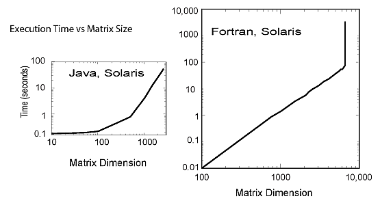
"As indicated in Figures 10.3 and 11.2, the data cache holds a copy of\n",
"some of the data in memory. The basics are the same for all caches, but\n",
"the sizes are manufacturer-dependent. When the CPU tries to address a\n",
"memory location, the *cache manager* checks to see if the data are in\n",
"the cache. If they are not, the manager reads the data from memory into\n",
"the cache, and then the CPU deals with the data directly in the cache.\n",
"The cache manager’s view of RAM is shown in Figure 11.2.\n",
"\n",
"When considering how a matrix operation uses memory, it is important to\n",
"consider the *stride* of that operation, that is, the number of array\n",
"elements that are stepped through as the operation repeats. For\n",
"instance, summing the diagonal elements of a matrix to form the trace\n",
"\n",
"$$\\tag*{11.7}\n",
"\\mbox{Tr} A = \\sum_{i=1}^{N}a(i,i)$$\n",
"\n",
"involves a large stride because the diagonal elements are stored far\n",
"apart for large *N*. However, the sum\n",
"\n",
"$$\\tag*{11.8} c(i) = x(i) + x(i+1)$$\n",
"\n",
"has stride 1 because adjacent elements of *x* are involved. The basic\n",
"rule in programming for a cache is\n",
"\n",
"- Keep the stride low, preferably at 1, which in practice means:\n",
"\n",
"- Vary the leftmost index first on Fortran arrays.\n",
"\n",
"- Vary the rightmost index first on Python and C arrays.\n",
"\n",
"### 11.4.1 Exercise 1: Cache Misses\n",
"\n",
"We have said a number of times that your program will be slowed down if\n",
"the data it needs are in virtual memory and not in RAM. Likewise, your\n",
"program will also be slowed down if the data required by the CPU are not\n",
"in the cache. For high-performance computing, you should write programs\n",
"that keep as much of the data being processed as possible in the cache.\n",
"To do this you should recall that Fortran matrices are stored in\n",
"successive memory locations with the row index varying most rapidly\n",
"(column-major order), while Python and C matrices are stored in\n",
"successive memory locations with the column index varying most rapidly\n",
"(row-major order). While it is difficult to isolate the effects of the\n",
"cache from other elements of the computer’s architecture, you should now\n",
"estimate its importance by comparing the time it takes to step through\n",
"the matrix elements row by row to the time it takes to step through the\n",
"matrix elements column by column.\n",
"\n",
"\n",
"\n",
" **Figure 11.2** The cache manager’s view of\n",
"RAM. Each 128-B cache line is read into one of four lines in cache.\n",
"\n",
"Run on machines available to you a version of each of the two simple\n",
"codes listed below. Check that although each has the same number of\n",
"arithmetic operations, one takes significantly more time to execute\n",
"because it makes large jumps through memory, with some of the memory\n",
"locations addressed not yet read into the cache:\n",
"\n",
"**Listing 11.10 Sequential column and row references.**\n",
"\n",
" for j = 1, 999999;\n",
" x(j) = m(1,j) // Sequential column reference\n",
"\n",
"\n",
"**Listing 11.11 Sequential column and row references.**\n",
"\n",
" for j = 1, 999999;\n",
" x(j) = m(j,1) // Sequential row reference\n",
"\n",
"### 11.4.2 Exercise 2: Cache Flow\n",
"\n",
"Below in Listings 11.12 and 11.13 we give two simple code fragments that\n",
"you should place into full programs in whatever computer language you\n",
"are using. Test the importance of cache flow on your machine by\n",
"comparing the time it takes to run these two programs. Run for\n",
"increasing column size `idim` and compare the times for loop $A$\n",
"*versus* those for loop $B$. A computer with very small caches may be\n",
"most sensitive to stride.\n",
"\n",
"**Listing 11.12 ** Loop A: GOOD f90 (min stride), BAD Python/C (max\n",
"stride)\n",
"\n",
" Dimension Vec(idim,jdim) // Stride 1 fetch (f90)\n",
" for j = 1, jdim; { for i=1, idim; Ans = Ans + Vec(i,j)*Vec(i,j)}\n",
"\n",
"**Listing 11.13 ** Loop B: BAD f90 (max stride), GOOD Python/C (min\n",
"stride)\n",
"\n",
" Dimension Vec(idim, jdim) // Stride jdim fetch (f90)\n",
" for i = 1, idim; {for j=1, jdim; Ans = Ans + Vec(i,j)*Vec(i,j)}\n",
"\n",
"Loop $A$ steps through the matrix `Vec` in column order. Loop $B$ steps\n",
"through in row order. By changing the size of the columns (the leftmost\n",
"Python index), we change the step size (*stride*) taken through memory.\n",
"Both loops take us through all the elements of the matrix, but the\n",
"stride is different. By increasing the stride in any language, we use\n",
"fewer elements already present in the cache, require additional swapping\n",
"and loading of the cache, and thereby slow down the whole process.\n",
"\n",
"### 11.4.3 Exercise 3: Large-Matrix Multiplication\n",
"\n",
"As you increase the dimensions of the arrays in your program, memory use\n",
"increases geometrically, and at some point you should be concerned about\n",
"efficient memory use. The penultimate example of memory usage is large-matrix\n",
"multiplication:\n",
"\n",
"$$\\begin{align} \\tag*{11.9}\n",
"[C] & = [A] \\times [B], \\\\\n",
" c_{ij} & = \\sum_{k=1}^{N} a_{ik}\n",
"\\times b_{kj}.\\tag*{11.10}\\end{align}$$\n",
"\n",
"**Listing 11.14 BAD f90 (max stride), GOOD Python/C (min stride)**\n",
"\n",
" for i = 1, N; { // Row\n",
" for j = 1, N; { // Column\n",
" c(i,j) = 0.0 // Initialize\n",
" for k = 1, N; {\n",
" c(i,j) = c(i,j) + a(i,k)*b(k,j) }}} // Accumulate\n",
"\n",
"This involves all the concerns with different kinds of memory. The\n",
"natural way to code (11.9) follows from the definition of matrix\n",
"multiplication (11.10), that is, as a sum over a row of $A$ times a\n",
"column of $B$. Try out the two codes in Listings 11.14 and 11.15 on your\n",
"computer. In Fortran, the first code uses matrix $B$ with stride 1, but\n",
"matrix $C$ with stride $N$. This is corrected in the second code by\n",
"performing the initialization in another loop. In Python and C, the\n",
"problems are reversed. On one of our machines we found a factor of 100\n",
"difference in CPU times despite the fact that the number of operations\n",
"is the same!\n",
"\n",
"**Listing 11.15 GOOD f90 (min stride), BAD Python/C (max stride)**\n",
"\n",
" for j = 1, N; { // Initialization\n",
" for i = 1, N; {\n",
" c(i,j) = 0.0 }\n",
" for k = 1, N; {\n",
" for i = 1, N; {c(i,j) = c(i,j) + a(i,k)*b(k,j) }}}\n",
"\n",
"\n",
"\n",
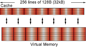
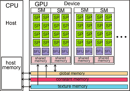
"**Figure 11.3** A schematic of a GPU (on the right) and its interactions with a\n",
"CPU (on the left). The GPU is seen to have streaming multiprocessors, special\n",
"function units and several levels of memory. Also shown is the communication\n",
"between memory levels and with the host CPU (on the left)."
]
},
{
"cell_type": "markdown",
"metadata": {},
"source": [
"## 11.5 Graphical Processing Units for High Performance Computing\n",
"\n",
"In §10.16 we discussed how the trend towards exascale computing appears\n",
"to be one using Multinode-Multicore-GPU Computers, as illustrated in\n",
"Figure 10.14. The GPU component in this figure extends a supercomputer’s\n",
"architecture beyond that of computers such as IBM Blue Gene. The GPU’s\n",
"in these future supercomputers are electronic devices designed to\n",
"accelerate the creation of visual images. A GPU’s efficiency arises from\n",
"its ability to create many different parts of an image in parallel, an\n",
"important ability because there are millions of pixels to display\n",
"simultaneously. Indeed, these units can process 100s of millions of\n",
"polygons in a second. Because GPU’s are designed to assist the video\n",
"processing on commodity devices such as personal computers, game\n",
"machines, and mobile phones, they have become inexpensive, high\n",
"performance, parallel computers in their own right. Yet because GPU’s\n",
"are designed to assist in video processing, their architecture and their\n",
"programming are different from that of the general purpose CPU’s usually\n",
"used for scientific applications, and it takes some work to use them for\n",
"scientific computing.\n",
"\n",
"Programming of GPU’s requires specialized tools specific to the GPU\n",
"architecture being used, and while we do discuss them in § 11.6.2, their\n",
"low-level details places it beyond the normal level of this book. What\n",
"is often called “CUDA programming” refers to programming for the\n",
"architecture developed by the Nvidia corporation, and is probably the\n",
"most popular approach to GPU programming at present \\[Zeller(08)\\].\n",
"However, some of the complications are being reduced via extensions and\n",
"wrappers developed for popular programming languages such as C, Fortran,\n",
"Python, Java and Perl. However, the general principles involved are just\n",
"an extension of those used already discussed, and after we have you work\n",
"through some examples of those general principles, in §11.6 we give some\n",
"practical tips for programming multinode-multicore-GPU computers.\n",
"\n",
"In the [Chapter 10](CP10.ipynb) we discussed some high-level aspects\n",
"regarding parallel computing. In this section we discuss some practical\n",
"tips for multicore, GPU programming. In the next section we provide some\n",
"actual examples of GPU programming using Nvidia’s *CUDA* language, with\n",
"access to it from within Python programs via the use of *PyCUDA*\n",
"\\[Klöckner(14)\\]. But do not think this is nothing more than adding in\n",
"another package to Python. That section is marked as optional because\n",
"using CUDA goes beyond the usual level of this text, and because, in our\n",
"experience, it can be difficult for a regular scientist to get CUDA\n",
"running on their personal computer without help. As is too often the\n",
"case with parallel computing, one does have to get one’s hands dirty\n",
"with lower-level commands. Our presentation should give the reader some\n",
"general understanding of CUDA. To read more on the subject, we recommend\n",
"the CUDA tutorial \\[[Zeller(08))](BiblioLinked.html#cuda4)\\], as well as \\[[Kirk & Wen-Mei(13))](BiblioLinked.html#cuda1),\n",
"[Sanders & Kandrot(11))](BiblioLinked.html#cuda2), [Faber(10))](BiblioLinked.html#cuda3)\\].\n",
"\n",
"### 11.5.1 The GPU Card\n",
"\n",
"GPU’s are hardware components that are designed to accelerate the\n",
"storage, manipulation and display of visual images. GPU’s tend to have\n",
"more core chips and more arithmetic data processing units than do\n",
"multicore central processing units (CPU’s), and so are essentially fast,\n",
"but limited, parallel computers. Because GPU’s have become commodity\n",
"items on most PC’s (think gaming), they hold the promise of being a\n",
"high-powered, yet inexpensive, parallel computing environment. At\n",
"present an increasing number of scientific applications are being\n",
"adapted to GPU’s, with the CPU used for the sequential part of a program\n",
"and the GPU for the parallel part.\n",
"\n",
"The most popular GPU programming language is ’s CUDA (Compute Unified\n",
"Device Architecture). CUDA is both a platform and a programming model\n",
"created by Nvidia for parallel computing on their GPU. The model\n",
"defines:\n",
"\n",
"1. threads, clocks and grids,\n",
"\n",
"2. a memory system with registers, local, shared and global memories,\n",
" and\n",
"\n",
"3. an execution environment with scheduling of threads and blocks\n",
" of threads.\n",
"\n",
"Figure 11.3 shows a schematic of a typical Nvidia card containing four\n",
"streaming multiprocessors (SMs), each with eight streaming processors\n",
"(SP’s), two special function units (SFUs), and 16 KB of shared memory.\n",
"The SFUs are used for the evaluation of the, otherwise, time-consuming\n",
"transcendental functions such as sin, cosine, reciprocal, and square\n",
"root. Each group of dual SMs form a texture processing cluster (TPC)\n",
"that is used for pixel shading or general-purpose graphical processing.\n",
"Also represented in the figure is the transfer of data among the three\n",
"types of memory structures on the GPU and those on the host (on the\n",
"left). Having memory on the chip is much faster than accessing remote\n",
"memory structures."
]
},
{
"cell_type": "markdown",
"metadata": {},
"source": [
"## 11.6 Practical Tips for Multicore & GPU Programming$\\odot$\n",
"\n",
"We have already described some basic elements of exascale computing in\n",
"§10.16. Some practical tips for programming multinode-multicore-GPU\n",
"computers follow along the same lines as we have been discussing, but\n",
"with an even greater emphasis on minimizing communication costs\\[*Note:*\n",
"Much of the material in this section comes from talks by John Dongarra\n",
"\\[Dongarra(11)\\].\\]. Contrary to the traditional view on optimization,\n",
"this means that the “faster” of two algorithms may be the one that takes\n",
"more steps, but requires less communications. Because the effort in\n",
"programming the GPU directly can be quite high, many application\n",
"programmers prefer to let compiler extensions and wrappers deal with the\n",
"GPU. But if you must, here’s how.\n",
"\n",
"Exascale computers and computing are expected to be *“disruptive\n",
"technologies”* in that they lead to drastic changes from previous models\n",
"for computers and computing. This is in contrast to the more evolving\n",
"technology of continually increasing the clock speed of the CPU, which\n",
"was the practice until the power consumption and associated heat\n",
"production imposed a roadblock. Accordingly, we should expect that\n",
"software and algorithms will be changing (and we will have to rewrite\n",
"our applications), much as it did when supercomputers changed from large\n",
"vector machines with proprietary CPU’s to cluster computers using\n",
"commodity CPU’s and message passing. Here are some of the major points\n",
"to consider:\n",
"\n",
"Exacascale data movement is expensive\n",
"\n",
": The time for a floating-point operation and for a data transfer can\n",
" be similar, although if the transfer is not local, as Figures 10.12\n",
" and 10.14 show happens quite often, then communication will be the\n",
" rate-limiting step.\n",
"\n",
"Exacascale flops are cheap and abundant\n",
"\n",
": GPU’s and local multicore chips provide many, very fast flops for us\n",
" to use, and we can expect even more of these elements to be included\n",
" in future computers. So do not worry about flops as much\n",
" as communication.\n",
"\n",
"Synchronization-reducing algorithms are essential\n",
"\n",
": Having many processors stop in order to synchronize with each other,\n",
" while essential in ensuring that the proper calculation is being\n",
" performed, can slow down processing to a halt (literally). It is\n",
" better to find or derive an algorithm that reduces the need\n",
" for synchronization.\n",
"\n",
"Break the fork-join model\n",
"\n",
": This model for parallel computing takes a queue of incoming jobs,\n",
" divides them into subjobs for service on a variety of servers, and\n",
" then combines them to produce the final result. Clearly, this type\n",
" of model can lead to completed subjobs on various parts of the\n",
" computer that must wait for other subjobs to complete\n",
" before recombination. A big waste of resources.\n",
"\n",
"Communication-reducing algorithms\n",
"\n",
": As already discussed, it is best to use methods that lessen the need\n",
" for communication among processors, even if more flops are needed.\n",
"\n",
"Use mixed precision methods\n",
"\n",
": Most GPU’s do not have native double precision floating-point\n",
" numbers (or even full single precision) and correspondingly slow\n",
" down by a factor-of-two or more when made to perform double\n",
" precision calculation, or when made to move double-precision data.\n",
" The preferred approach then is to use single precision. One way to\n",
" do this is to utilize perturbation theory in which the calculation\n",
" focuses on the small (single precision) correction to a known, or\n",
" separately calculated, large (double precision) basic solution. The\n",
" rule-of-thumb then is to use the lowest precision required to\n",
" achieve the required accuracy.\n",
"\n",
"Push for and use autotuning\n",
"\n",
": The computer manufactures have advanced the hardware to incredible\n",
" speeds, but have not produced concordant advances in the software\n",
" that scientists need to utilize in order to make good use of\n",
" these machines. It often takes people-years to rewrite a large\n",
" program for these new machines, and that is a tremendous investment\n",
" that not many scientists can afford. We need smarter software to\n",
" deal with such complicated machines, and tools that permit us to\n",
" optimize experimentally our programs for these machines.\n",
"\n",
"Fault resilient algorithms\n",
"\n",
": Computers containing millions or billions of components do make\n",
" mistakes at times. It does not make sense to have to start a\n",
" calculation over, or hold a calculation up, when some minor failure\n",
" such as a bit flip occurs. The algorithms should be able to recover\n",
" from these types of failures.\n",
"\n",
"Reproducibility of results\n",
"\n",
": Science is at its heart the search for scientific truth, and there\n",
" should be only one answer when solving a problem whose solution is\n",
" mathematically unique. However, approximations in the name of speed\n",
" are sometimes made and this can lead to results whose exact\n",
" reproducibility cannot be guaranteed. (Of course exact\n",
" reproducibility is not to be expected for Monte Carlo calculations\n",
" involving chance.)\n",
"\n",
"Data layout is critical\n",
"\n",
": As we discussed with Figures 10.3, 11.2 and 11.4, much of HPC deals\n",
" with matrices and their arrangements in memory. With parallel\n",
" computing we must arrange the data into tiles such that each data\n",
" tile is contiguous in memory. Then the tiles can be processed in a\n",
" fine-grained computation. As we have seen in the exercises, the best\n",
" size for the tiles depends upon the size of the caches being used,\n",
" and these are generally small.\n",
"\n",
"\n",
"\n",
"**Figure 11.4** A schematic of how the contiguous elements of a matrix must\n",
"be tiled for parallel processing (from \\[Dongarra(11)\\]).\n",
"\n",
"### 11.6.1 CUDA Memory Usage\n",
"\n",
"CUDA commands are extensions of the C programming language and are used\n",
"to control the interaction between the GPU’s components. CUDA supports\n",
"several data types such as dim2, dim3 and 2-D textures, for 2-D, 3-D and\n",
"2-D shaded objects respectively. PyCUDA \\[Klöckner(14)\\], in turn,\n",
"provides access to CUDA from Python programs as well as providing some\n",
"additional extensions of C. Key concepts when programming with CUDA are\n",
"the\n",
"\n",
"Kernel:\n",
"\n",
": a part or parts of a program that are executed in parallel by the\n",
" GPU using threads. The kernel is called from the host and executed\n",
" on the *device* (another term for the GPU).\n",
"\n",
"Thread:\n",
"\n",
": the basic element of data to be processed on the GPU. Sometimes\n",
" defined as an execution of a kernel with a given index, or the\n",
" abstraction of a function call acting on data. The numbers of\n",
" threads that are able to run concurrently on a GPU depends upon the\n",
" specific hardware being used.\n",
"\n",
"Index:\n",
"\n",
": All threads see the same kernel, but each kernel is executed with a\n",
" different parameter or subscript, called an index.\n",
"\n",
"As a working example, consider the summation of the arrays `a` and `b`\n",
"by a kernel with the result assigned to the array `c`:\n",
"\n",
"$$\\tag*{11.11}\n",
" c_i = a_i + b_i.$$\n",
"\n",
"If this were calculated using a sequential programming model, then we\n",
"might use a `for` loop to sum over the index `i`. However, this is not\n",
"necessary in CUDA where each thread sees the same kernel, but there is a\n",
"different ID assigned to each thread. Accordingly, one thread associated\n",
"with an ID would see:\n",
"\n",
"$$\\tag*{11.12} c_0= a_0+ b_0,$$\n",
"\n",
"while another thread asssigned to a different ID might see:\n",
"\n",
"$$\\tag*{11.13} c_1= a_1+ b_1,$$\n",
"\n",
"and so forth. In this way the summation is performed in parallel by the\n",
"GPU. You can think of this model as analogous to an orchestra in which\n",
"all violins plays the same part with the conductor setting the timing\n",
"(the clock cycles in the computer). Each violinist has the same sheet\n",
"music (the kernel) yet plays his/her own violin (the threads).\n",
"\n",
"As we have already seen in Figure 11.3, CUDA’s GPU architecture contains\n",
"scalable arrays of multithreaded streaming multiprocesors (SMs). Each SM\n",
"contains eight streaming processors (SP), also called CUDA cores, and\n",
"these are the parts of the GPU that run the kernels. The SPs are\n",
"execution cores like CPU’s, but simpler. They typically can perform more\n",
"operations in a clock cycle than the CPU, and being dedicated just to\n",
"data processing, constitute the Arithmetic Logic Units (ALU) of the GPU.\n",
"The speed of dedicated SM’s, along with their working in parallel, leads\n",
"to the significant processing power of GPU’s, even when compared to a\n",
"multicore CPU computer.\n",
"\n",
"In the CUDA approach, the threads are assigned in *blocks* that can\n",
"accommodate from one to thousands of threads. For example, the CUDA\n",
"GeForce GT 540M can handle 1024 threads per block, and has 96 cores. As\n",
"we have said, each thread runs the same program, which make this a\n",
"single program multiple data computer. The threads of a block are\n",
"partitioned into *warps* (set of lengthwise yarns in weaving), with each\n",
"warp containing 32 threads. The blocks can be 1-D, 2-D or 3-D, and are\n",
"organized into *grids*. The grids, in turn, can be 1-D or 2-D.\n",
"\n",
"When a grid is created or *launched*, the blocks are assigned to the\n",
"streaming multiprocessors in an arbitrary order, with each block\n",
"partitioned into warps, and each thread going to a different streaming\n",
"processor. If more blocks are assigned to an SM than it can process at\n",
"once, the excess blocks are scheduled for a later time. For example, the\n",
"GT200 architecture can process 8 blocks or 1024 threads per SM, and\n",
"contain 30 SMs. This means that the 8$\\times $30 = 240 CUDA\n",
"cores (SPs) can process 30$\\times$1024 = 30,720 threads in\n",
"parallel. Compare that to a 16 core CPU!"
]
},
{
"cell_type": "markdown",
"metadata": {},
"source": [
"### 11.6.2 CUDA Programming$\\odot$\n",
"\n",
"The installation of CUDA development tools follows a number of steps:\n",
"\n",
"1. Establish that the video card on your system has a GPU with\n",
" Nvidia CUDA. Just having an Nvidia card might not do because not all\n",
" Nvidia cards have a CUDA architecture.\n",
"\n",
"2. Verify that your operating system can support CUDA and PyCuda (Linux\n",
" seems to be the preferred system).\n",
"\n",
"3. On Linux, verify that your system has gcc installed. On Windows, you\n",
" will need the Microsoft Visual Studio compiler.\n",
"\n",
"4. Download the Nvidia CUDA Toolkit.\n",
"\n",
"5. Install the Nvidia CUDA Toolkit.\n",
"\n",
"6. Test that the installed software runs and can communicate with\n",
" the CPU.\n",
"\n",
"7. Establish that your Python environment contains PyCuda. If not,\n",
" install it.\n",
"\n",
"Let’s now return to our problem of summing two arrays and storing the\n",
"result, `a[i]+b[i]=c[i]`. The steps needed to solve this problem using a\n",
"host (CPU) and a device (GPU) are:\n",
"\n",
"1. Declare single precision arrays in the host and initialize\n",
" the arrays.\n",
"\n",
"2. Reserve space in the device memory to accommodate the arrays.\n",
"\n",
"3. Transfer the arrays from the host to the device.\n",
"\n",
"4. Define a kernel on the host to sum the arrays, with the execution of\n",
" the kernel to be performed on the device.\n",
"\n",
"5. Perform the sum on the device, transfer the result to the host and\n",
" print it out.\n",
"\n",
"6. Finally, free up the memory space on the device.\n",
"\n",
"[**Listing 11.16 ** The PyCUDA program **SumArraysCuda.py**](http://www.science.oregonstate.edu/~rubin/Books/CPbook/Codes/HPCodes/SumArraysCuda.py) uses the GPU\n",
"to do the array sum a + b = c.\n",
"\n",
"Listing 11.16 presents a PyCUDA program `SummArraysCuda.py` that\n",
"performs our array summation on the GPU. The program is seen to start on\n",
"line 3 with the `import pycuda.autoinit` command that initializes CUDA\n",
"to accept the kernel. Line 4, `import pycuda.driver as drv`, is needed\n",
"for Pycuda to be able to find the available GPU. Line 7,\n",
"`from pycuda.compiler import SourceModule` prepares the Nvidia kernel\n",
"compiler `nvcc`. The `SourceModule`, which nvcc compiles, is given in\n",
"CUDA C on lines 10-14.\n",
"\n",
"As indicated before, even though we are summing indexed arrays, there is\n",
"no explicit `for` loop running over an index i. This is\n",
"because CUDA and the hardware know about arrays and so take care of the\n",
"indices automatically. This works by having all threads seeing the same\n",
"kernel, and also by having each thread process a different value of `i`.\n",
"Specifically, notice the command `const int i = threadIdx.x` on line 11\n",
"in the source module. The suffix `.x` indicates that we have a one\n",
"dimensional collections of threads. If we had a 2-D or 3D collection,\n",
"you would also need to include `threadIdx.y` and `threadIdx.z` commands.\n",
"Also notice in this same SourceModule the prefix `global` on line 11.\n",
"This indicates that the execution of the following summation is to be\n",
"spread among the processors on the device.\n",
"\n",
"\n",
"\n",
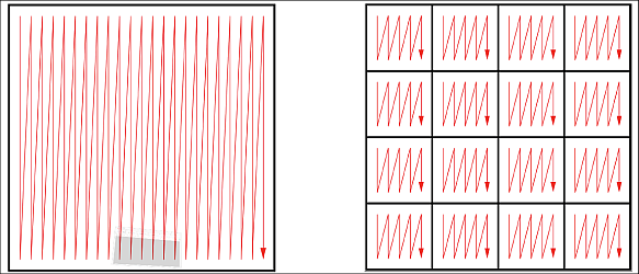
"**Figure 11.5** *Top:* A $1\\times1$ grid with a 1-D block containing 32\n",
"threads, and the corresponding threadIdx.x that goes from 0 to 31. *Bottom:* A\n",
"1-D $4\\times1$ grid, that has 4 blocks with 8 threads each.\n",
"\n",
"In contrast to Python, where arrays are double precision floating-point\n",
"numbers, in CUDA arrays are single precision. Accordingly, on lines 17\n",
"and 18 of Listing 11.16 we specify the type of arrays with the command\\\n",
"`a = numpy.array(range(N)).astype(numpy.float32)`.\\\n",
"The prefix `numpy` indicates where the `array` data type is defined,\n",
"while the suffix indicates that the array is single precision (32 bits).\n",
"Next on lines 22-24 are the `drv.memalloc(a.nbytes)` statements needed\n",
"to reserve memory on the device for the arrays. With `a` already\n",
"defined, `a.nbytes` translates into the number of bytes in the array.\n",
"After that, the `drv.memcphtod()` commands are used to copy `a` and `b`\n",
"to the device. The sum is performed with the `sumab()` command, and then\n",
"the result is sent back to the host for printing.\n",
"\n",
"Several of these steps can be compressed by using some PyCUDA-specific\n",
"commands. Specifically, the memory allocation, the performance of the\n",
"summation and the transmission of the results on lines 22-28 can be\n",
"replaced by the statements\n",
"\n",
" sum_ab(\n",
" drv.Out(c), drv.In(a), drv.In(b),\n",
" block=(N,1,1), grid=(1,1)) # a, b sent to device, c to host\n",
"\n",
"with the rest of the program remaining the same. The statement\n",
"`grid=(1,1)` describes the dimension of the grid in blocks as 1 in x and\n",
"1 in y, which is the same as saying that the grid is composed of one\n",
"block. The `block(N,1,1)` command indicates that there are `N` (=32)\n",
"threads, with the `1,1` indicating that the threads are only in the x\n",
"direction.\n",
"\n",
"[**Listing 11.17 ** The PyCUDA program **SumArraysCuda2.py**](http://www.science.oregonstate.edu/~rubin/Books/CPbook/Codes/HPCodes/SumArraysCuda2.py) uses the\n",
"GPU to do the array sum a + b = c, using four blocks with a (4,1) grid.\n",
"\n",
"Our example is so simple that we have organized it into just a single\n",
"1-D block of 32 threads in a $1\\times 1$ grid (top of Figure 11.5).\n",
"However, in more complicated problems, it often makes sense to\n",
"distribute the threads over a number of different block, with each block\n",
"performing a different operation. For example, the program\n",
"`SumArraysCuda2.py` in Listing 11.17 performs the same sum with the\n",
"four-block structure illustrated on the bottom of Figure 11.5. The\n",
"difference in the program here is the statement on line 23,\n",
"`block=(8,1,1), grid=(4,1)` that specifies a grid of 4 blocks in 1-D x,\n",
"with each 1-D block having 8 threads. To use this structure of the\n",
"program, on line 10 we have the command\n",
"`const int i = threadIdx.x+blockDim.x*blockIdx.x;`. Here `blockDim.x` is\n",
"the dimension of each block in threads (8 in this case numbered 0, 1,\n",
"...,7), with `blockIdx.x` indicating the block numbering. The threads in\n",
"each block have `treadIdx.x` from 0 to 7 and the corresponding IDs of\n",
"the blocks are `blockIdx.x` =0, 1, 2 and 3."
]
},
{
"cell_type": "code",
"execution_count": null,
"metadata": {
"collapsed": true
},
"outputs": [],
"source": []
}
],
"metadata": {
"kernelspec": {
"display_name": "Python 2",
"language": "python",
"name": "python2"
},
"language_info": {
"codemirror_mode": {
"name": "ipython",
"version": 2
},
"file_extension": ".py",
"mimetype": "text/x-python",
"name": "python",
"nbconvert_exporter": "python",
"pygments_lexer": "ipython2",
"version": "2.7.11"
}
},
"nbformat": 4,
"nbformat_minor": 0
}