{
"cells": [
{
"cell_type": "markdown",
"metadata": {},
"source": [
"# *Chapter 14*
Nonlinear Population Dynamics \n",
"\n",
"| | | |\n",
"|:---:|:---:|:---:|\n",
"| 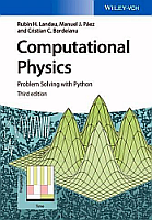|[From **COMPUTATIONAL PHYSICS**, 3rd Ed, 2015](http://physics.oregonstate.edu/~rubin/Books/CPbook/index.html)
RH Landau, MJ Paez, and CC Bordeianu (deceased)
Copyrights:
[Wiley-VCH, Berlin;](http://www.wiley-vch.de/publish/en/books/ISBN3-527-41315-4/) and [Wiley & Sons, New York](http://www.wiley.com/WileyCDA/WileyTitle/productCd-3527413154.html)
R Landau, Oregon State Unv,
MJ Paez, Univ Antioquia,
C Bordeianu, Univ Bucharest, 2015.
Support by National Science Foundation.||\n",
"\n",
"**14 Nonlinear Population Dynamics**
\n",
"[14.1 Bug Population Dynamics](#14.1)
\n",
"[14.2 The Logistic Map (Model)](#14.2)
\n",
"[14.3 Properties of Nonlinear Maps (Theory & Exercise)](#14.3)
\n",
" [14.3.1 Fixed Points](#14.3.1)
\n",
" [14.3.2 Period Doubling, Attractors](#14.3.3)
\n",
"[14.4 Mapping Implementation](#14.4)
\n",
"[14.5 Bifurcation Diagram](#14.5)
\n",
" [14.5.1 Implementation](#14.5.1)
\n",
" [14.5.2 Visualization Algorithm: Binning](#14.5.2)
\n",
" [14.5.3 Feigenbaum Constants (Exploration)](#14.5.3)
\n",
"[14.6 Logistic Map Random Numbers (Exploration)](#14.6)
\n",
"[14.7 Other Maps (Exploration)](#14.7)
\n",
"[14.8 Signals of Chaos: Lyapunov Coefficients & Shannon Entropy](#14.8)
\n",
"[14.9 Coupled Predator-Prey Models](#14.9)
\n",
"[14.10 Lotka-Volterra Model](#14.10)
\n",
"[14.10.1 Lotka-Volterra Assessment](#14.10.1)
\n",
"[14.11 Predator-Prey Chaos](#14.11)
\n",
" [14.11.1 Exercises](#14.11.1)
\n",
" [14.11.2 LVM with Prey Limit](#14.11.2)
\n",
" [14.11.3 LVM with Predation Efficiency](#14.11.3)
\n",
" [14.11.4 LVM Implementation and Assessment](#14.11.4)
\n",
" [14.11.5 Two Predators, One Prey](#14.11.5)\n",
"(Exploration)
\n",
"\n",
"*Nonlinear dynamics is one of the success stories of computational\n",
"physics. It has been explored by scientists and engineers with computers\n",
"as an essential tool, often then followed by mathematicians \\[[Motter &\n",
"Campbell(13)](BiblioLinked.html#motter)\\]. The computations have led to the discovery of new\n",
"phenomena such as solitons, chaos and fractals, as you will discover on\n",
"your own. In addition, because biological systems often have complex\n",
"interactions and may not be in thermodynamic equilibrium states, models\n",
"of them are often nonlinear, with properties similar to those of other\n",
"complex systems. In this chapter we look at discrete models of\n",
"population dynamics that are simple yet produce surprising complex\n",
"behavior. In the next chapter we explore chaos for continuous systems.*\n",
"\n",
"** This Chapter’s Lecture, Slide Web Links, Applets & Animations**\n",
"\n",
"| | |\n",
"|---|---|\n",
"|[All Lectures](http://physics.oregonstate.edu/~rubin/Books/CPbook/eBook/Lectures/index.html)|[](http://physics.oregonstate.edu/~rubin/Books/CPbook/eBook/Lectures/index.html)|\n",
"\n",
"| *Lecture (Flash)*| *Slides* | *Sections*|*Lecture (Flash)*| *Slides* | *Sections*| \n",
"|- - -|:- - -:|:- - -:|- - -|:- - -:|:- - -:|\n",
"|[Bugs](http://www.science.oregonstate.edu/~rubin/Books/CPbook/eBook/Lectures/Modules/Bugs/Bugs_ipad.mp4)|[pdf](http://science.oregonstate.edu/~rubin/Books/CPbook/eBook/Slides/Slides_NoAnimate_pdf/Bugs_18Dec09.pdf)|12.1|[Chaotic Pend I](http://www.science.oregonstate.edu/~rubin/Books/CPbook/eBook/Lectures/Modules/Chaos_I/Chaos_I_ipad.mp4)|[pdf](http://science.oregonstate.edu/~rubin/Books/CPbook/eBook/Slides/Slides_NoAnimate_pdf/Pend1_27Jan09.pdf)| 12.10 | \n",
"|[Chaotic Pend II](http://www.science.oregonstate.edu/~rubin/Books/CPbook/eBook/Lectures/Modules/Chaos_II/Chaos_II_ipad.mp4)|[pdf](http://science.oregonstate.edu/~rubin/Books/CPbook/eBook/Slides/Slides_NoAnimate_pdf/Pend2_07Jan09.pdf)| 12.12|[Chaotic Pend III](http://www.science.oregonstate.edu/~rubin/Books/CPbook/eBook/Lectures/Modules/Chaos_III/Chaos_III_ipad.mp4)|[pdf](http://science.oregonstate.edu/~rubin/Books/CPbook/eBook/Slides/Slides_NoAnimate_pdf/Pend3_07Jan09.pdf)| 12.14| \n",
"| [Chaotic Pendulum Applet](http://science.oregonstate.edu/~rubin/Books/CPbook/eBook/Applets/index.html)|-|12.11|[Hypersensitive Pendula Applet](http://www.science.oregonstate.edu/~rubin/Books/CPbook/eBook/Applets/index.html)|-| 12.11| \n",
"|[Double Pendulum Movie](http://www.science.oregonstate.edu/~rubin/Books/CPbook/eBook/Applets/index.html)|-|12.14 |[Classical Chaotic Scattering Applet](http://www.science.oregonstate.edu/~rubin/Books/CPbook/eBook/Applets/index.html)|-|9.14| \n",
"|[HearData: Data2Sound Applet](http://www.science.oregonstate.edu/~rubin/Books/CPbook/eBook/Applets/index.html)|-|12.13|[Lissajous Figures Applet](http://www.science.oregonstate.edu/~rubin/Books/CPbook/eBook/Applets/index.html)|-| 12.12|\n",
"|[Visualizing with Sound Applet](http://www.science.oregonstate.edu/~rubin/Books/CPbook/eBook/Applets/index.html)|- |12.13| | |"
]
},
{
"cell_type": "markdown",
"metadata": {},
"source": [
"## 14.1 Bug Population Dynamics \n",
"\n",
"**Problem:** Populations of insects and patterns of weather do not\n",
"appear to follow any simple laws \\[*note:* Except maybe in Oregon, where\n",
"storm clouds come to spend their weekends.\\]. At times the populations\n",
"patterns appear stable, at other times they vary periodically, and at\n",
"other times they appear chaotic, with no discernable regularity, only to\n",
"settle down to something simple again. Your **problem** is to deduce if\n",
"a simple law can produce such complicated behaviors.\n",
"\n",
"## 14.2 The Logistic Map (Model) \n",
"\n",
"Imagine a bunch of insects reproducing generation after generation. We\n",
"start with $N_0$ bugs, then in the next generation we have to live with\n",
"$N_1$ of them, and after $i$ generations there are $N_i$ bugs to bug us.\n",
"We want to define a model of how $N_n$ varies with the discrete\n",
"generation number $n$. Clearly, if the rates of breeding and dying are\n",
"the same, then a stable population should occur. Yet bugs cannot live on\n",
"love alone, they must also eat, and bugs not being farmers must compete\n",
"for the available food supply. This tends to restrict their number to\n",
"lie below some maximum population. We want to build these observations\n",
"into our model.\n",
"\n",
"For guidance, we look to the radioactive decay simulation in [Chapter\n",
"4](CP04.ipynb), *Monte Carlo: Randomness, Walks & Decays*, where the\n",
"discrete decay law, $\\Delta N/\\Delta t = -\\lambda N$, led to exponential-like\n",
"decay.Likewise, if we reverse the sign of $\\lambda$, we should get\n",
"exponential-like *growth*, which is a good place to start our modelling. We\n",
"assume that the bug-breeding rate is proportional to the number of bugs:\n",
"\n",
"$$\\tag*{14.1}\n",
"\\frac{\\Delta N_i}{\\Delta t} = \\lambda \\; N_i.$$ Because we know the\n",
"empirical fact that exponential growth usually tapers off, we extend the model\n",
"by incorporating the observation that for a given environment there must be\n",
"maximum population $N_{*}$, which is called the *carrying capacity*.\n",
"Consequently, we modify the exponential growth model (14.1) by modifying the\n",
"growth rate so that it decreases as the population $N_i$ approaches $N_{*}$:\n",
"\n",
"$$\\begin{align}\n",
"\\tag*{14.2}\n",
"\\lambda &\\rightarrow \\lambda' (N_*-N_i)\\\\\n",
" \\Rightarrow \\ \\frac{\\Delta\n",
"N_i}{\\Delta t} & = \\lambda'(N_{*}-N_i)N_i.\\tag*{14.3}\n",
" \\end{align}$$\n",
" \n",
" We expect that when $N_i$ is small compared to $N_*$,\n",
"the population will grow exponentially. We also expect that as $N_i$\n",
"approaches $N_*$, the growth rate will decrease, eventually becoming\n",
"negative if $N_i$ exceeds the carrying capacity $N_*$.\n",
"\n",
"Equation (14.3) is a form of the *logistic map*. It is usually written as a relation\n",
"between the number of bugs in future and present generations:\n",
"\n",
"$$\\begin{align}\n",
"\\tag*{14.4}\n",
"N_{i+1} & = N_i + \\lambda' \\Delta t (N_{*}-N_i)N_i ,\\\\ & = N_i\\left(1 + \\lambda'\n",
"\\Delta t N_{*} \\right) \\left[1 -\\frac{\\lambda' \\Delta t} {1+\\lambda' \\Delta t\n",
"N_{*}}N_i\\right]. \\tag*{14.5}\\end{align}$$\n",
"\n",
"This relation looks simpler when\n",
"expressed in terms of dimensionless variables:\n",
"\n",
"$$\\begin{align}\\tag*{14.6}\n",
" x_{i+1} &= \\mu x_{i}(1- x_{i}), \\\\\n",
" \\mu & \\stackrel{\\rm def}{\\ \\ =\\ \\ } 1 + \\lambda' \\Delta t N_{*}, \\tag*{14.7}\\\\\n",
"x_{i} & \\stackrel{\\rm def}{\\ \\ =\\ \\ } \\frac{\\lambda' \\Delta t}{1 + \\lambda' \\Delta t N_{*}} N_i\\simeq\n",
"\\frac{N_i}{N_{*}}.\\tag*{14.8}\n",
" \\end{align}$$\n",
" \n",
" Here $\\mu$ is a dimensionless growth parameter and\n",
"$x_{i}$ is a dimensionless population variable. Observe from (14.6) that\n",
"the *growth rate* $\\mu =1$ when the breeding rate $\\lambda'$ equals $0$,\n",
"and is otherwise expected to be larger than 1. If the number of bugs\n",
"born per generation $\\lambda' \\Delta t$ is large, then\n",
"$\\mu \\simeq \\lambda' \\Delta t N_{*}$ and $x_{i} \\simeq\n",
"N_i/N_{*}$, that is, $x_{i}$ is essentially the fraction of the maximum\n",
"population $N_{*}$. Consequently, realistic $x$ values generally lie in\n",
"the range $0 \\leq x_{i} \\leq 1$, with $x=0$ corresponding to no bugs,\n",
"and $x=1$ corresponding to the maximum population.\n",
"\n",
"The map (14.6) is seen to be the sum of a linear and a quadratic dependence on\n",
"$x_i$. In general, we employ the term “map” to refer to a function $f(x)$ that\n",
"converts one number in a sequence to the next, $$\\tag*{14.9} x_{i+1} = f(x_{i})\n",
".$$ For the logistic map, $f(x) = \\mu x (1-x)$, with the quadratic dependence on\n",
"$x$ making this a nonlinear map, and the dependence on only the one variable\n",
"$x$ making it a *one-dimensional* map.\n",
"\n",
"Just by looking at (14.6) there is no way of knowing how good a model\n",
"this will be. Being as simple as it is, the model cannot be expected to\n",
"be a complete description of the population dynamics of bugs. However,\n",
"if it exhibits some features similar to those found in nature, then it\n",
"may well form the foundation for a more complete description.\n",
"\n",
"\n",
"\n",
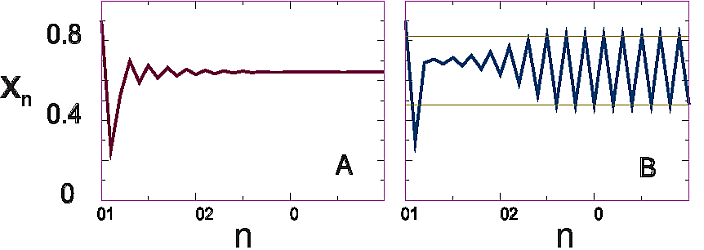
"**Figure 14.1** The insect population $\\textit{x}_{\\text{n}}$ *versus* the\n",
"generation number $\\textit{n}$ for the two growth rates: (A) $\\mu =\n",
"\\text{2.8}$, a single attractor; (B) $\\mu = \\text{3.3}$, a double attractor.\n"
]
},
{
"cell_type": "markdown",
"metadata": {},
"source": [
"## 14.3 Properties of Nonlinear Maps (Theory & Exercise) \n",
"\n",
"Rather than going through some fancy mathematical analysis to learn\n",
"about the properties of the logistic map \\[[Rasband(90)](BiblioLinked.html#rash)\\], we suggest\n",
"that you explore it yourself on a computer or a calculator by generating\n",
"and plotting sequences of $x_i$ values. You should get results similar\n",
"to those shown in Figures 14.1 and 14.2.\n",
"\n",
"**Stable Populations** We want to see if the model can produce a stable\n",
"population, that is, one that remains the same from generation to\n",
"generation.\n",
"\n",
"1. Calculate and plot $x_{i+1}$ as a function of the generation number\n",
" $i$.\n",
"\n",
"2. The initial population $x_0$ is called the *seed*, and we suggest\n",
" $x_0=0.75$ as a good starting value (the dynamical effects are not\n",
" sensitive to the seed).\n",
"\n",
"3. Your results should be highly sensitive to the value for the growth\n",
" rate $\\mu$. Too large a value may lead to instabilities, while too\n",
" small a value may lead to extinction. To make sure that the model is\n",
" behaving reasonably, try some cases for which we can be fairly sure\n",
" of what the results should be. By trying some negative and zero\n",
" values for $\\mu$ (for example, -1, -0.75, -0.5, -0.25, 0) we should\n",
" obtain decaying populations.\n",
"\n",
"4. Now that you have some confidence in the model, see if you can\n",
" increase the population to some stable values. With the same initial\n",
" population as before, try $\\mu$ = 0, 0.5, 1.0, 1.5, 2. Make plots of\n",
" $x_i$ versus $i$ for each of these cases.\n",
"\n",
"5. Take note of the *transient* behavior in these plots that occur for\n",
" early generations before a steady state or more regular behavior\n",
" sets in. In general, these are not the long-term dynamical behaviors\n",
" of interest.\n",
"\n",
"6. For a fixed value of $\\mu$, try different values for the seed\n",
" population $x_0$. Verify that differing values of $x_0$ do affect\n",
" the transients, but *not* the values of the stable populations.\n",
"\n",
"You should have found that with positive growth rates $\\mu$, this model\n",
"yields stable populations, with the bugs approaching the maximum\n",
"population more rapidly as $\\mu$ gets larger. This is a good validation\n",
"of the model. Some typical behaviors are shown in Figures 14.1 and 14.2\n",
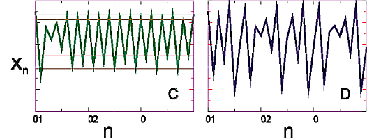
". In Figure 14.1A we see equilibration into a single population; in\n",
"Figure 14.2A we see oscillation between two population levels; in\n",
"14.2C we see oscillation among four levels; and in 14.2B we\n",
"see a chaotic system.\n",
"\n",
"\n",
"\n",
"**Figure 14.2** The insect population $\\textit{x}_{\\text{n}}$ *versus* the\n",
"generation number $\\textit{n}$ for two different growth rates: (C) $\\mu =\n",
"\\text{3.5}$, a quadruple attractor; (D) $\\mu= \\text{3.8}$, a chaotic regime.\n",
"\n",
"### 14.3.1 Fixed Points\n",
"\n",
"An important property of the map (14.6) is the possibility of the\n",
"sequence $x_{i}$ reaching a *fixed* point $x_{*}$, that is, a value of\n",
"the population at which the system remains. At a *one-cycle*\n",
"fixed-point, there is no change in the population from generation $i$ to\n",
"generation $i+1$, that is,\n",
"\n",
"$$\\tag*{14.10} x_{i+1} = x_{i} = x_{*}.$$\n",
"\n",
"Substituting the logistic map (14.6) into this equation produces an\n",
"algebraic equation that we can solve:\n",
"\n",
"$$\\begin{align}\n",
"\\tag*{14.11}\n",
"\\mu x_{*} (1-x_{*}) & = x_{*}, \\\\\n",
" \\Rightarrow \\quad x_{*} & = 0, \\qquad \\frac{\\mu -\n",
"1}{\\mu}.\\tag*{14.12}\n",
" \\end{align}$$\n",
"\n",
"The nonzero fixed-point $x_{*}=(\\mu - 1)/\\mu$ corresponds to a stable\n",
"population with a balance between birth and death that is reached regardless of\n",
"the initial population (Figure 14.1A). In contrast, the $x_{*} = 0$ point is\n",
"unstable and the population remains static only as long as no bugs exist; if even\n",
"a few bugs are introduced, exponential growth occurs. Further analysis (§14.8)\n",
"tells us that the stability of a population is determined by the magnitude of the\n",
"derivative of the mapping function $f(x_{i})$ at the fixed-point \\[Rasband(90)\\]:\n",
"\n",
"$$\\begin{align}\n",
"\\tag*{14.13}\n",
"\\left| \\frac{df}{dx}\\right|_{x_{*}} < 1 \\quad \\mbox{(stable)}.\\end{align}$$\n",
"\n",
"For the one cycle of the logistic map (14.6), the derivative is\n",
"\n",
"$$\\tag*{14.14}\n",
"\\left.\\frac{df}{dx}\\right|_{x_{*}} = \\mu - 2 \\mu x_{*} =\n",
"\\begin{cases}\n",
"\\mu, &\\mbox{stable at}\\ x_{*} = 0\\ \\mbox{if }\\ \\mu<1, \\\\\n",
"2-\\mu, & \\mbox{stable at}\\ x_{*} = \\frac{\\mu-1} {\\mu} \\ \\mbox{if }\\ \\mu < 3.\n",
"\\end{cases}$$\n",
"\n",
"### 14.3.2 Period Doubling, Attractors\n",
"\n",
"Equation (14.14) tells us that while the equation for fixed-points (14.11) may be\n",
"satisfied for all values of $\\mu$, the populations will not be stable if $\\mu >3$.\n",
"In this latter case, the system’s long-term population *bifurcates* into two\n",
"populations, a so called *two-cycle*. The effect is known as *period doubling*\n",
"and is evident in Figure 14.1B. Because the system now acts as if it were\n",
"attracted to two populations, these populations are called *attractors* or\n",
"*cycle points*. We can easily predict the $x$ values for these two-cycle\n",
"attractors by demanding that generation $i+2$ have the same population as\n",
"generation $i$:\n",
"\n",
"$$\\begin{align}\n",
"\\tag*{14.15}\n",
"x_{i} & = x_{i+2} = \\mu x_{i+1}(1-x_{i+1})\\\\\n",
"\\Rightarrow \\quad x_{*} & = \\frac{1+\\mu \\pm \\sqrt{\\mu^{2}-2\\mu -\n",
"3}}{2\\mu}.\\tag*{14.16}\n",
" \\end{align}$$\n",
" \n",
" We see that as long as $\\mu>3$, the square root\n",
"produces a real number and thus that physical solutions exist (complex\n",
"or negative $x_*$ values are nonphysical). We leave it to your computer\n",
"explorations to discover how the system continues to double periods as\n",
"$\\mu$ is further increased. In all cases the pattern repeats: one\n",
"populations bifurcates into two."
]
},
{
"cell_type": "markdown",
"metadata": {},
"source": [
"## 14.4 Mapping Implementation \n",
"\n",
"It is now time to carry out a more careful investigation of the logistic\n",
"map along the original path followed by \\[[Feigenbaum(79)](BiblioLinked.html#feig)\\]:\n",
"\n",
"1. Confirm Feigenbaum’s observations of the different patterns shown in\n",
" Figures 14.1 and 14.2 that occur for\n",
" $\\mu = (0.4, 2.4, 3.2, 3.6, 3.8304)$ and seed $x_{0}= 0.75$.\n",
"\n",
"2. Identify the following in your graphs:\n",
"\n",
"3. **Transients:** Irregular behaviors before reaching a steady state\n",
" that differ for different seeds.\n",
"\n",
"4. **Asymptotes:** In some cases the steady state is reached after only\n",
" 20 generations, while for larger $\\mu$ values, hundreds of\n",
" generations may be needed. These steady-state populations are\n",
" independent of the seed.\n",
"\n",
"5. **Extinction:** If the growth rate is too low, $\\mu\\le 1$, the\n",
" population dies off.\n",
"\n",
"6. **Stable states:** The stable single-population states attained for\n",
" $\\mu<3$ should agree with the prediction (14.11).\n",
"\n",
"7. **Multiple cycles:** Examine the map orbits for a growth parameter\n",
" $\\mu$ increasing continuously through 3. Observe how the system\n",
" continues to double periods as $\\mu$ increases. To illustrate, in\n",
" Figure 14.2C with $\\mu = 3.5$, we notice a steady state in which the\n",
" population alternates among four attractors (a *four-cycle*).\n",
"\n",
"8. **Intermittency:** Observe simulations for $ 3.8264 < \\mu <\n",
" 3.8304$. Here the system appears stable for a finite number of\n",
" generations and then jumps all around, only to become stable again.\n",
"\n",
"9. **Chaos:** *We define chaos as the deterministic behavior of a\n",
" system displaying no discernible regularity.* This may seem\n",
" contradictory; if a system is deterministic, it must have\n",
" step-to-step correlations (which, when added up, mean long-range\n",
" correlations); but if it is chaotic, the complexity of the behavior\n",
" may hide the simplicity within. In an operational sense, a chaotic\n",
" system is one with an extremely high sensitivity to parameters or\n",
" initial conditions. This sensitivity to even minuscule changes is so\n",
" high that it is impossible to predict the long-range behavior unless\n",
" the parameters are known to infinite precision (a\n",
" physical impossibility).\n",
"\n",
"10. The system’s behavior in the chaotic region is critically dependent\n",
" on the exact values of $\\mu$ and $x_0$. Systems starting out with\n",
" nearly identical values for $\\mu$ and $x_0$ may end up with quite\n",
" different behaviors. In some cases the complicated behaviors of\n",
" nonlinear systems will be *chaotic*, but this is not the same as\n",
" being random.\\[*Note:* You may recall from [Chapter 4, *Monte Carlo:\n",
" Randomness, Walks & Decays*](CP04.ipynb), that a truly random\n",
" sequence of events does not even have next step predictability,\n",
" while these chaotic systems do.\\]\n",
"\n",
"11. Compare the long-term behaviors of starting with the two essentially\n",
" identical seeds $x_0= 0.75$ and $x_0' = 0.75 (1 +\n",
" \\epsilon)$, where $\\epsilon \\simeq 2 \\times 10^{-14}$.\n",
"\n",
"12. Repeat the simulation with $x_0= 0.75$ and two essentially identical\n",
" survival parameters, $ \\mu = 4.0$ and $\\mu' = 4.0 (1 -\n",
" \\epsilon)$, where $\\epsilon \\simeq 2 \\times 10^{-14}$. Both\n",
" simulations should start off the same but eventually diverge."
]
},
{
"cell_type": "markdown",
"metadata": {},
"source": [
"## 14.5 Bifurcation Diagram (Assessment) \n",
"\n",
"Watching the population change with generation number gives a good idea\n",
"of the basic dynamics, at least until it gets too complicated to discern\n",
"patterns. In particular, as the number of bifurcations keeps increasing\n",
"and the system becomes chaotic, it may be hard to see a simple\n",
"underlying structure within the complicated behavior. One way to\n",
"visualize what is going on is to concentrate on the attractors, that is,\n",
"those populations that appear to attract the solutions and to which the\n",
"solutions continuously return (long-term iterates). A plot of these\n",
"attractors of the logistic map as a function of the growth parameter\n",
"$\\mu$ is an elegant way to summarize the results of extensive computer\n",
"simulations.\n",
"\n",
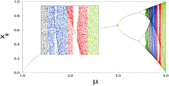
"A *bifurcation diagram* for the logistic map is shown in Figure 14.3,\n",
"with one for a Gaussian map given in Figure 14.4. To generate such a\n",
"diagram you proceed through all values of $\\mu$ in steps. For each value\n",
"of $\\mu$, you let the system go through hundreds of iterations to\n",
"establish that the transients have died out, and then write the values\n",
"$(\\mu,x_{*})$ to a file for hundreds of iterations after that. If the\n",
"system falls into an $n$-cycle for this $\\mu$ value, then there should\n",
"predominantly be $n$ different values written to the file. Next, the\n",
"value of the initial populations $x_0$ is changed slightly, and the\n",
"entire procedure is repeated to ensure that no fixed-points are missed.\n",
"When finished, your program will have stepped through all the values of\n",
"$\\mu$ and $x_0$. Our sample program `Bugs.py` is shown in Listing 14.1.\n",
"\n",
"[**Listing 14.1 Bugs.py**](http://www.science.oregonstate.edu/~rubin/Books/CPbook/Codes/PythonCodes/Bugs.py) produces the bifurcation diagram of the logistic map.\n",
"A full program requires finer grids, a scan over initial values, and removal of\n",
"duplicates."
]
},
{
"cell_type": "code",
"execution_count": null,
"metadata": {
"collapsed": true
},
"outputs": [],
"source": [
"### Bugs.py, Notebook Version"
]
},
{
"cell_type": "code",
"execution_count": null,
"metadata": {
"collapsed": true
},
"outputs": [],
"source": [
"# Bugs.py, Noitebook Version, Logistic map\n",
"\n",
"from IPython.display import IFrame\n",
"from numpy import *\n",
"import numpy as np\n",
"import matplotlib.pyplot as plt\n",
"\n",
"m_min = 1.0\n",
"m_max = 4.0\n",
"step = 0.01\n",
"lasty = int(1000 * 0.5) # to eliminate later some points\n",
"count = 0 # to plot later every two iterations\n",
"for m in arange(m_min, m_max, step):\n",
" y = 0.5\n",
" for i in range(1,201,1): #to avoid transients\n",
" y = m*y*(1-y) \n",
" for i in range(201,402,1):\n",
" y = m*y*( 1 - y) \n",
" for i in range(201, 402, 1): # to avoid transients\n",
" oldy=int(1000*y)\n",
" y = m*y*(1 - y) \n",
" inty = int(1000 * y)\n",
" if inty != lasty and count%2 == 0:\n",
" plt.plot(m,y,'bo',markersize=1) # to avoid repeats\n",
" lasty = inty\n",
" count += 1\n",
"\n",
"plt.show()"
]
},
{
"cell_type": "markdown",
"metadata": {},
"source": [
"### 14.5.1 Bifurcation Diagram Implementation\n",
"\n",
"The last part of this problem asks you to reproduce Figure 14.3 at\n",
"various levels of detail. While the best way to make a visualization of\n",
"this sort would be with visualization software that permits you to vary\n",
"the intensity of each individual point on the screen, we simply plot\n",
"individual points and have the density in each region determined by the\n",
"number of points plotted there. When thinking about plotting many\n",
"individual points to draw a figure, it is important to keep in mind that\n",
"your monitor may have approximately 100 pixels per inch and your laser\n",
"printer 300 dots per inch. This means that if you plot a point at each\n",
"pixel, you will be plotting\n",
"${\\sim} 3000 \\times 3000 {\\simeq} 10$ million elements. *Beware:*\n",
"This can require some time and may choke a printer. In any case,\n",
"printing at a finer resolution is a waste of time.\n",
"\n",
"\n",
"\n",
"**Figure 14.3** A bifurcation plot of attractor population $x^{*}$\n",
"*versus* growth rate $\\mu$ for the logistic map. The inset\n",
"shows some details of a three-cycle window. (The colors or grey scales indicate\n",
"the regimes over which we distributed the work on different CPU’s when run in\n",
"parallel.)\n",
"\n",
"\n",
"\n",
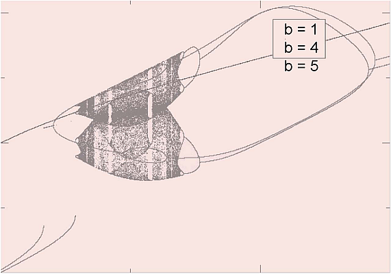
"**Figure 14.4** A bifurcation plot for the Gaussian map $f(x)=\\exp(-bx^2) +\n",
"\\mu$. (Courtesy of W. Hager.)\n",
"\n",
"### 14.5.2 Visualization Algorithm: Binning\n",
"\n",
"1. Break up the range $1 \\leq \\mu \\leq 4$ into 1000 steps. These are\n",
" the “bins” into which we will place the $x_*$ values.\n",
"\n",
"2. In order not to miss any structures in your bifurcation diagram,\n",
" loop through a range of initial $x_0$ values as well.\n",
"\n",
"3. Wait at least 200 generations for the transients to die out, and\n",
" then print the next several hundred values of $(\\mu,x_{*})$ to\n",
" a file.\n",
"\n",
"4. Print out your $x_{*}$ values to no more than three or four\n",
" decimal places. You will not be able to resolve more places than\n",
" this on your plot, and this restriction will keep your output files\n",
" smaller, as will removing duplicate entries. You can use formatted\n",
" output to control the number of decimal places, or you can do via a\n",
" simple conversion: multiply the $x_i$ values by 1000 and then throw\n",
" away the part to the right of the decimal point:\\\n",
" `Ix[i]= int(1000*x[i]) `\\\n",
" You may then divide by 1000 if you want floating-point numbers.\n",
"\n",
"5. Plot your file of $x_{*}$ *versus* $\\mu$. Use small\n",
" symbols for the points and do not connect them.\n",
"\n",
"6. Enlarge (zoom in on) sections of your plot and notice that a similar\n",
" bifurcation diagram tends to be contained within each magnified\n",
" portion (this is called *self-similarity*).\n",
"\n",
"7. Look over the series of bifurcations occurring at\n",
"\n",
" $$\\tag*{14.17}\n",
" \\mu_{k} \\simeq 3, 3.449, 3.544, 3.5644, 3.5688,\n",
" 3.569692, 3.56989, \\ldots .$$\n",
"\n",
" The end of this series is a region of chaotic behavior.\n",
"\n",
"8. Inspect the way this and other sequences begin and then end\n",
" in chaos. The changes sometimes occur quickly, and so you may have\n",
" to make plots over a very small range of $\\mu$ values to see\n",
" the structures.\n",
"\n",
"9. A close examination of Figure 14.3 shows regions where, for a slight\n",
" increase in $\\mu$, a very large number of populations suddenly\n",
" change to very few populations. Whereas these may appear to be\n",
" artifacts of the video display, this is a real effect and these\n",
" regions are called *windows*. Check that at $\\mu=3.828427$ chaos\n",
" moves into a three-cycle population.\n",
"\n",
"### 14.5.3 Feigenbaum Constants (Exploration)\n",
"\n",
"Feigenbaum discovered that the sequence of $\\mu_{k}$ values (14.17) at which\n",
"bifurcations occur follows a regular pattern \\[Feigenbaum(79)\\]. Specifically,\n",
"the $\\mu$ values converge geometrically when expressed in terms of the\n",
"distance between bifurcations $\\delta$:\n",
"\n",
"$$\\begin{align}\n",
"\\tag*{14.18}\n",
"\\mu_{k} & \\ \\rightarrow \\ \\mu_{\\infty} -\n",
"\\frac{c}{\\delta^{k}},\\\\\n",
"\\delta & = \\lim_{k\\rightarrow \\infty}\n",
"\\frac{\\mu_{k} - \\mu_{k-1}}{\\mu_{k+1} - \\mu_{k}}.\\tag*{14.19}\\end{align}$$\n",
"\n",
"Use your sequence of $\\mu_{k}$ values to determine the constants in\n",
"(14.18) and compare them to those found by Feigenbaum:\n",
"\n",
"$$\\tag*{14.20}\n",
"\\mu_{\\infty} \\simeq 3.56995, \\quad c \\simeq 2.637, \\quad \\delta\n",
"\\simeq 4.6692.$$\n",
"\n",
"Amazingly, the value of the *Feigenbaum constant* $\\delta$ is universal\n",
"for all second-order maps."
]
},
{
"cell_type": "markdown",
"metadata": {},
"source": [
"## 14.6 Logistic Map Random Numbers (Exploration) $\\odot$\n",
"\n",
"Although we have emphasized that chaos, with its short-term predictability, is\n",
"different from random, with has no predictability, it is nevertheless possible for\n",
"the logistic map in the chaotic region ($\\mu \\geq 4$) to be used to generate\n",
"pseudo random numbers \\[[Phatak & Rao(95)](BiblioLinked.html#shashi)\\]. This is carried out in two steps:\n",
"\n",
"$$\\begin{align}\n",
"\\tag*{14.21}\n",
"x_{i+1} & \\simeq 4 x_{i}(1-x_{i}),\\\\\n",
"y_{i} & = \\frac{1}{\\pi}\n",
"\\cos^{-1}(1-2x_{i}).\\tag*{14.22}\\end{align}$$\n",
"\n",
"Although successive $x_i$’s are\n",
"correlated, if the population for every sixth generation or so is examined, the\n",
"correlation is effectively gone and pseudorandom numbers result. To make the\n",
"sequence more uniform, the trigonometric transformation is then used.\n",
"\n",
"**Exercise:** Use the random-number tests discussed in [Chapter 4,\n",
"*Monte Carlo: Randomness, Walks & Decays*](CP04.ipynb), or an actual\n",
"Monte Carlo simulation, to test this claim.\n",
"\n",
"## 14.7 Other Maps (Exploration) \n",
"\n",
"Bifurcations and chaos are characteristic properties of nonlinear\n",
"systems. Yet systems can be nonlinear in a number of ways. The table\n",
"below lists four maps that generate $x_{i}$ sequences containing\n",
"bifurcations.\n",
"\n",
"|**Map Name** | $f(x)$ |**Map Name** | $f(x)$| \n",
"|- - -|- - -|- - -|- - -|\n",
"|Logistic| $\\mu x(1-x)$| Tent | $\\mu (1- 2\\left|x-1/2\\right|)$|\n",
"|Ecology | $x e^{\\mu(1-x)}$|Quartic | $\\mu [1-(2x-1)^{4}]$|\n",
"|Gaussian | $ e^{-b x^2} + \\mu$||| \n",
"\n",
"The tent map derives its nonlinear dependence from the absolute\n",
"value operator, while the logistic map is a subclass of the ecology map. Explore\n",
"the properties of these other maps and note the similarities and differences."
]
},
{
"cell_type": "markdown",
"metadata": {},
"source": [
"## 14.8 Signals of Chaos: Lyapunov Coefficient & Shannon Entropy$\\odot$ \n",
"\n",
"The Lyapunov coefficient or exponent $\\lambda_i$ provides an analytic\n",
"measure of whether a system is chaotic \\[[Wolf et al(85)](BiblioLinked.html#Wolf), [Ramasubramanian &\n",
"Sriram(00)](BiblioLinked.html#Ramasub), [Williams(97)](BiblioLinked.html#Williams)\\]. Essentially, the coefficient is a measure of the rate of\n",
"exponential growth of the solution near an attractor. If the coefficient is positive\n",
"then the solution moves away from the attractor, which is an indication of\n",
"chaos, while if the coefficient is negative then the solution moves back toward\n",
"the attractor, which is an indication of stability. For 1-D problems there is only\n",
"one such coefficient, whereas in general there is a coefficient for each degree of\n",
"freedom. The essential assumption is that the distance $L(t)$ between\n",
"neighboring paths $x_n$ at time $t$ near an attractor have an $n$ (generation\n",
"number or time) dependence $L \\propto \\exp(\\lambda t)$. Consequently, orbits\n",
"that have $\\lambda >0$ diverge and are chaotic; orbits that have $\\lambda =0$\n",
"remain marginally stable, while orbits with $\\lambda <0$ are periodic and\n",
"stable. Mathematically, the Lyapunov coefficient is defined as\n",
"\n",
"$$\\begin{align}\n",
"\\tag*{14.23}\n",
"\\lambda=\\lim_{t\\to \\infty} \\frac{1 }{t} \\log\n",
"\\frac{L(t)}{L(t_0)}.\\end{align}$$\n",
"\n",
"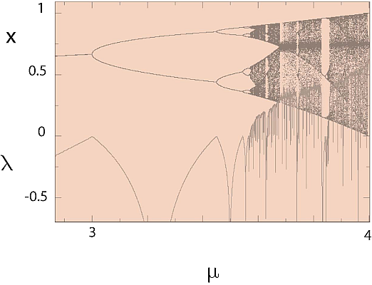 **Figure 14.5** Bifurcation values (top) and\n",
"Lyapunov coefficients (bottom) forthe logistic map as functions of the\n",
"growth rate $\\mu$. Notice how the Lyapunov coefficient, whose value is a\n",
"measure of chaos, changes abruptly at the bifurcations.\n",
"\n",
"As an example, we calculate the Lyapunov exponent for a general 1-D map,\n",
"\n",
"$$\\tag*{14.24} x_{n+1}=f(x_n),$$\n",
"\n",
"and then apply the result to the logistic map. To determine stability,\n",
"we examine perturbations about a reference trajectory $x_0$ by adding a\n",
"small perturbation and iterating once \\[[Manneville(90)](BiblioLinked.html#Manneville), [Ramasubramanian\n",
"& Sriram(00)](BiblioLinked.html#Ramasub)\\]:\n",
"\n",
"$$\\tag*{14.25}\n",
"\\hat{x}_0 =x_0+\\delta x_0, \\quad \\hat{x}_1 =x_1+\\delta\n",
"x_1.$$\n",
"\n",
"We substitute this into (14.24) and expand $f$ in a Taylor series around\n",
"$x_0$:\n",
"\n",
"$$\\begin{align} \n",
"x_1+\\delta x_1 &= f(x_0+\\delta x_0) \\simeq f(x_0)+ \\left.\n",
"\\frac{\\delta f}{\\delta x}\\right|_{x_0} \\delta x_0 =\n",
"x_1+\\left. \\frac{\\delta f}{\\delta x}\\right|_{x_0} \\delta x_0, \\\\\n",
"\\Rightarrow\\quad \\delta x_1 &\\simeq \\left(\\frac{\\delta f}{\\delta x}\\right)_{x_0}\\delta x_0.\\tag*{14.26}\\end{align}$$\n",
"\n",
"This is the proof of our earlier statement that a negative derivative\n",
"indicates stability. To deduce the general result we examine one\n",
"iteration:\n",
"\n",
"$$\\begin{align}\n",
"\\tag*{14.27}\n",
"\\delta x_2 &\\simeq \\left(\\frac{\\delta f}{\\delta\n",
"x}\\right)_{x_1}\\quad \\delta x_1 = \\left( \\frac{\\delta f}{\\delta\n",
"x}\\right)_{x_0}\\left(\\frac{\\delta f}{\\delta x}\\right)_{x_1}\\delta x_0,\\\\\n",
"\\Rightarrow\\quad \\delta x_n &=\n",
"\\prod_{i=0}^{n-1}\\left(\\frac{\\delta f}{\\delta\n",
"x}\\right)_{x_i}\\delta x_0.\\tag*{14.28}\\end{align}$$\n",
"\n",
"This last relation tells us how trajectories differ on the average after\n",
"$n$ steps:\n",
"\n",
"$$\\tag*{14.29} |\\delta x_n| =L^n |\\delta x_0|,\\quad L^n =\\prod_{i=0}^{n-1}\\left|\n",
"\\left(\\frac{\\delta f}{\\delta x}\\right)_{x_i}\\right|.$$\n",
"\n",
"We now solve for the Lyapunov number $L$ and take its logarithm to\n",
"obtain the Lyapunov coefficient:\n",
"\n",
"$$\\tag*{14.30}\n",
"\\lambda =\\ln(L)=\\lim_{n\\rightarrow \\infty} \n",
"\\frac{1}{n}\\sum_{i=0}^{n-1}\\ln \\left|\\left(\\frac{\\delta f}{\\delta x}\\right)_{x_i}\\right|.$$\n",
"\n",
"For the logistic map we obtain\n",
"\n",
"$$\\tag*{14.31}\n",
"\\lambda =\\frac{1}{n}\\sum_{i=0}^{n-1} \\ln|mu -2\\mu\n",
"x_i|,$$\n",
"\n",
"where the sum is over iterations.\n",
"\n",
"The code `LyapLog.py` in Listing 14.2 computes the Lyapunov exponents\n",
"for the bifurcation plot of the logistic map. In Figures 14.5 and 14.6\n",
"we show its output, and note the sign changes in $\\lambda$ where the\n",
"system becomes chaotic, and the abrupt changes in slope at bifurcations.\n",
"(A similar curve is obtained for the fractal dimension of the logistic\n",
"map as, indeed, the two are proportional.)"
]
},
{
"cell_type": "markdown",
"metadata": {},
"source": [
"### LyapLog.py, Notebook Version"
]
},
{
"cell_type": "code",
"execution_count": null,
"metadata": {
"collapsed": true
},
"outputs": [],
"source": [
"# LyapLog.py, Notebook Version, Lyapunov coef for logistic map\n",
"\n",
"from IPython.display import IFrame\n",
"from numpy import *\n",
"import numpy as np\n",
"import matplotlib.pyplot as plt\n",
"\n",
"m_min = 2.1\n",
"m_max = 4.0\n",
"step = 0.05\n",
"yy=[]\n",
"xx=[]\n",
"\n",
"for m in arange(m_min, m_max, step): # m loop\n",
" y = 0.5\n",
" suma = 0.0\n",
" for i in range(1, 401, 1): \n",
" y = m*y*(1 - y) # Skip transients \n",
" for i in range(402, 601, 1):\n",
" y = m*y*(1 - y)\n",
" plt.plot(m, y ,'ro',markersize=1)\n",
" suma = suma + log(abs(m*(1. - 2.*y) )) # Lyapunov\n",
" suma=suma/401\n",
" xx=xx+[m]\n",
" yy=yy+[suma]\n",
" plt.plot(xx, yy) # Normalize\n",
" \n",
"plt.show() "
]
},
{
"cell_type": "markdown",
"metadata": {},
"source": [
"**Shannon entropy**, like the Lyapunov exponent, is used an indicator of\n",
"chaos.Entropy is a measure of uncertainty (garbled signal) that has\n",
"proven useful in communication theory \\[[Shannon(48)](BiblioLinked.html#Shannon), [Ott(02)](BiblioLinked.html#Ott), [Gould et\n",
"al.(06)](BiblioLinked.html#GTC)\\]. Imagine that an experiment has $N$ possible outcomes. If the\n",
"probability of each is $p_1, p_2,\\ldots ,p_N$, with normalization such\n",
"that $ \\sum_{i=1}^N p_i=1$, then the Shannon entropy is defined as\n",
"\n",
"$$\\tag*{14.32} S_{\\text{Shannon}}=-\\sum_{i=1}^N p_i ln p_i.$$\n",
"\n",
"[**Listing 14.2 LyapLog.py**](http://www.science.oregonstate.edu/~rubin/Books/CPbook/Codes/PythonCodes/Fractals/LyapLog.py) computes Lyapunov exponents for the bifurcation plot of\n",
"the logistic map as a function of growth rate. Note the fineness of the $\\mu$\n",
"grid. If $p_i \\equiv 0$, there is no uncertainty and $S_{\\text{Shannon}} = 0$, as\n",
"you might expect. If all $N$ outcomes have equal probability, $p_i \\equiv 1/N$,\n",
"we obtain the expression familiar from statistical mechanics,\n",
"$S_{\\text{Shannon}} = \\ln N$.\n",
"\n",
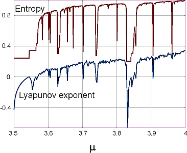
"The code `Entropy.py` in Listing 14.3 computes the Shannon entropy for\n",
"the logistic map as a function of the growth parameter $\\mu$. The\n",
"results (Figure 14.6 top) are seen to be quite similar to the Lyapunov\n",
"exponent, again with discontinuities occurring at the bifurcations.\n",
"\n",
"\n",
"\n",
"**Figure 14.6** Shannon entropy (top) and Lyapunov coefficient (bottom) for\n",
"the logistic map. Notice the close relation between the thermodynamic measure\n",
"of disorder (entropy) and the nonlinear dynamics measure of chaos (Lyapunov).\n",
"\n",
"[**Listing 14.3 Entropy.py**](http://www.science.oregonstate.edu/~rubin/Books/CPbook/Codes/PythonCodes/Fractals/Entropy.py) computes the Shannon entropy for the logistic\n",
"map as a function of growth parameter $\\mu$."
]
},
{
"cell_type": "markdown",
"metadata": {},
"source": [
"### Entropy.py, Notebook Version"
]
},
{
"cell_type": "code",
"execution_count": null,
"metadata": {
"collapsed": false
},
"outputs": [],
"source": [
"# Entropy.py, Notebook Version, Shannon Entropy for Logistic map\n",
"\n",
"from IPython.display import IFrame\n",
"from numpy import *\n",
"import numpy as np\n",
"import matplotlib.pyplot as plt\n",
"\n",
"mumin = 3.5\n",
"mumax = 4.0\n",
"dmu = 0.005\n",
"nbin = 1000\n",
"nmax = 100000\n",
"prob = zeros( (1000), float) \n",
"xx=[]\n",
"yy=[]\n",
"# first coord. mu0, entr0\n",
"for mu in arange(mumin, mumax, dmu): # mu loop\n",
" print(\"waiting until mu=4 before plotting \",mu)\n",
" for j in range(1, nbin):\n",
" prob[j] = 0\n",
" y = 0.5\n",
" for n in range(1, nmax + 1):\n",
" y = mu*y*(1.0 - y) # Logistic map, Skip transients\n",
" if (n > 30000):\n",
" ibin = int(y*nbin) + 1\n",
" prob[ibin] += 1\n",
" entropy = 0.\n",
" for ibin in range(1, nbin):\n",
" if (prob[ibin]>0):\n",
" entropy = entropy - (prob[ibin]/nmax)*math.log10(prob[ibin]/nmax)\n",
" yy=yy+[entropy] \n",
" xx=xx+[mu]\n",
" \n",
"plt.plot(xx,yy) \n",
"plt.title(\"Entropy vs $\\mu$\")\n",
"plt.xlabel('$\\mu$')\n",
"plt.show() "
]
},
{
"cell_type": "markdown",
"metadata": {},
"source": [
"## 14.9 Coupled Predator-Prey Models \n",
"\n",
"*At the beginning of this chapter we saw complicated behavior arising\n",
"from a model of bug population dynamics in which we imposed a maximum\n",
"population. We described that system with a discrete logistic map. Now\n",
"we study models describing predator-prey population dynamics proposed by\n",
"an American physical chemist \\[[Lotka(25)](BiblioLinked.html#lot)\\] and an Italian\n",
"mathematician \\[[Volterra(26)](BiblioLinked.html#volt), [[Gurney & Nisbet(98)\\]. Though\n",
"simple, versions of these equations are used to model biological systems\n",
"and neural networks.*\n",
"\n",
"**Problem:** Is it possible to use a small number of predators to\n",
"control a population of pests so that the number of pests remains\n",
"essentially constant? Include in your considerations the interaction\n",
"between the populations as well as the competition for food and\n",
"predation time.\n",
"\n",
"## 14.10 Lotka-Volterra Model \n",
"\n",
"We extend the logistic map to the Lotka-Volterra Model (LVM) which\n",
"describes two populations coexisting in the same geographical region.\n",
"Let\n",
"\n",
"$$\\tag*{14.33} p(t) = \\mbox{prey density}, \\qquad P(t)= \\mbox{Predator\n",
"density}.$$\n",
"\n",
"In the absence of interactions between the species, we assume that the\n",
"prey population $p$ breeds at a per-capita rate of $a$. This would lead\n",
"to exponential growth:\n",
"\n",
"$$\\begin{align}\n",
"\\tag*{14.34}\n",
"\\frac{\\Delta p}{\\Delta t} & = ap \\quad (\\mbox{Discrete}), \\\\\n",
"\\frac{dp}{dt} &= ap, \\quad (\\mbox{Continuous}),\\tag*{14.35}\\\\\n",
" \\Rightarrow \\quad p(t) &= p(0)e^{at}.\\tag*{14.36}\\end{align}$$\n",
"\n",
"Here we give both the discrete and continuous versions of the model,\n",
"with the exponential the solution of the continuous version. Yet\n",
"exponential growth does not occur because the predators $P$ eat more\n",
"prey if the number of prey increases. The interaction rate between\n",
"predator and prey requires both to be present, with the simplest\n",
"assumption being that it is proportional to their joint probability:\n",
"\n",
"$$\\begin{align}\n",
"\\tag*{14.37}\n",
"\\mbox{Interaction rate} = b p P ,\\end{align}$$\n",
"\n",
"where $b$ is a constant. This leads to a prey growth rate including both\n",
"predation and breeding:\n",
"\n",
" $$\\tag*{14.38}\n",
"\\frac{\\Delta p}{\\Delta t} = a p-b p P, \\quad\n",
"\\mbox{(Discrete LVM-I for prey)},$$\n",
"\n",
"$$\\tag*{14.39}\n",
" \\boxed{\\frac{dp}{dt} = a p-b p P, \\quad\n",
"\\mbox{(LVM-I for prey)}.}$$\n",
"\n",
"If left to themselves, predators $P$ will also breed and increase their\n",
"population. Yet predators need animals to eat, and if there are no other\n",
"populations to prey upon, we assume that they will eat each other (or\n",
"their young) at a per-capita mortality rate $m$:\n",
"\n",
"$$\\tag*{14.40}\n",
"\\left.\\frac{dP}{dt}\\right|_{\\textrm competition}= -mP, \\ \n",
"\\Rightarrow\\ P(t)=P(0)e^{-mt}.$$\n",
"\n",
"However, if there are prey also to interact with (read “eat”) at the\n",
"rate $b p P$, the predator population will grow at the rate\n",
"\n",
"$$\\tag*{14.41}\n",
" \\boxed{\\frac{dP}{dt} =\\epsilon b p P -m P \\qquad \\mbox{(LVM-I for predators)},}$$\n",
"\n",
"where $\\epsilon$ is a constant that measures the efficiency with which\n",
"predators convert prey interactions into food.\n",
"\n",
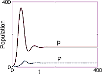
"|A|B| \n",
"|:- - -:|:- - -:|\n",
"|||\n",
"\n",
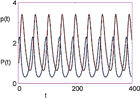
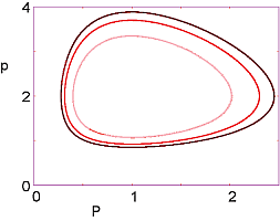
"**Figure 14.7** *A:* The time dependencies of the populations of prey *p(t)*\n",
"(solid curve) and of predator *P(t)* (dashed curve) from the Lotka-Volterra\n",
"model. *B:* A phase space plot of Prey population *p* as a function of\n",
"predator population $\\textit{P}$. The different orbits correspond to different\n",
"initial conditions.\n",
"\n",
"Equations (14.39) and (14.41) are two simultaneous ODE’s and are our first\n",
"model. After placing them in the standard dynamic form, we solve them with\n",
"the `rk4` algorithm:\n",
"\n",
"$$\\tag*{14.42}\n",
"\\begin{array}{r@{\\ }lcr@{\\ }l}\n",
"& &d\\mathbf{y}/dt= \\mathbf{f}(\\mathbf{y},t),&&\\\\ y_0 &= p, &&f_0 &= a y_0 - b\n",
"y_0 y_1,\\\\ y_1 &= P, &&f_1 &= \\epsilon b y_0 y_1 - m y_1.\n",
"\\end{array}$$\n",
"\n",
"A sample code to solve these equations is `PredatorPrey.py` in\n",
"Listing 14.4.\n",
"\n",
"[**Listing 14.4 PredatorPrey.py**](http://www.science.oregonstate.edu/~rubin/Books/CPbook/Codes/PythonCodes/PredatorPrey.py) computes the population dynamics for a\n",
"group of predators and prey."
]
},
{
"cell_type": "code",
"execution_count": null,
"metadata": {
"collapsed": true
},
"outputs": [],
"source": [
"### PredatorPrey.py, Notebook Version"
]
},
{
"cell_type": "code",
"execution_count": null,
"metadata": {
"collapsed": true
},
"outputs": [],
"source": [
"### PredatorPrey.py, Notebook Version\n",
"\n",
"from __future__ import division,print_function\n",
"from IPython.display import IFrame\n",
"from numpy import *\n",
"\n",
"import numpy as np\n",
"import matplotlib.pyplot as plt\n",
"\n",
"Tmin = 0.0\n",
"Tmax = 500.0 # endpoints\n",
"y = np.zeros( (2), float)\n",
"yy0=np.zeros((1002),float)\n",
"yy1=np.zeros((1002),float)\n",
"Ntimes = 1000\n",
"y[0] = 2.0\n",
"y[1] = 1.3 # initialize\n",
"h = (Tmax - Tmin)/Ntimes \n",
"t = Tmin\n",
"\n",
"def f( t, y, F): # FUNCTION of your choice here\n",
" F[0] = 0.2*y[0]*(1 - (y[0]/(20.0) )) - 0.1*y[0]*y[1] # RHS of 1st eq\n",
" F[1] = - 0.1*y[1] + 0.1*y[0]*y[1]; # RHS of 2nd eq\n",
" \n",
"def rk4(t, y, h, Neqs): # rk4 method, *DO NOT MODIFY*, instead, modify f\n",
" F = np.zeros( (Neqs), float)\n",
" ydumb = np.zeros( (Neqs), float)\n",
" k1 = np.zeros( (Neqs), float)\n",
" k2 = np.zeros( (Neqs), float)\n",
" k3 = np.zeros( (Neqs), float)\n",
" k4 = np.zeros( (Neqs), float)\n",
" f(t, y, F)\n",
" for i in range(0, Neqs):\n",
" k1[i] = h*F[i]\n",
" ydumb[i] = y[i] + k1[i]/2.\n",
" f(t + h/2., ydumb, F)\n",
" for i in range(0, Neqs):\n",
" k2[i] = h*F[i]\n",
" ydumb[i] = y[i] + k2[i]/2.\n",
" f(t + h/2., ydumb, F)\n",
" for i in range(0, Neqs):\n",
" k3[i] = h*F[i]\n",
" ydumb[i] = y[i] + k3[i]\n",
" f(t + h, ydumb, F)\n",
" for i in range(0, Neqs):\n",
" k4[i] = h*F[i]\n",
" y[i] = y[i] + (k1[i] + 2.*(k2[i] + k3[i]) + k4[i])/6.\n",
"tt=np.arange(0,Tmax+1,h)\t\t\t\t\n",
"#plt.plot(t,)\n",
"j=0\n",
"for t in np.arange(Tmin, Tmax + 1, h):\n",
" yy0[j]=y[0]\n",
" yy1[j]=y[1]\n",
" #print(j)\n",
" #funct1.plot(pos = (t, y[0]) )\n",
" #funct2.plot(pos = (t, y[1]) )\n",
" #funct3.plot(pos = (y[0], y[1]) )\n",
" #rate(60)\n",
" rk4(t, y, h, 2)\n",
" j+=1\n",
"plt.figure(0) \n",
"plt.plot(tt,yy0)\n",
"plt.title('Prey population p(green) and predator population P(blue) vs. time')\n",
"plt.ylabel('P,p')\n",
"plt.xlabel('t')\n",
"plt.plot(tt,yy1)\n",
"plt.figure(1)\n",
"plt.plot(yy0,yy1,'r')\n",
"plt.title('Predator population (P) vs prey (p) population')\n",
"plt.xlabel('p')\n",
"plt.ylabel('P')\n",
"\n",
"plt.show()"
]
},
{
"cell_type": "markdown",
"metadata": {},
"source": [
"### 14.10.1 Lotka-Volterra Assessment\n",
"\n",
"Results from the code `PredatorPrey.py` are shown in Figure 14.7. On the\n",
"left we see that the two populations oscillate out of phase with each\n",
"other in time; when there are many prey, the predator population eats\n",
"them and grows; yet then the predators face a decreased food supply and\n",
"so their population decreases; that in turn permits the prey population\n",
"to grow, and so forth. On the right in Figure 14.7 we plot what is\n",
"called a “phase space” plot of $P(t)$ *versus* $p(t)$. A closed orbit\n",
"here indicates a limit cycle that repeats indefinitely. Although\n",
"increasing the initial number of predators does decrease the maximum\n",
"number of pests, it is not a satisfactory solution to our **problem**,\n",
"as the large variation in the number of pests cannot be called\n",
"“control”.\n",
"\n",
"1. Explain in words why their is a correlation between extremums in\n",
" prey and predator populations?\n",
"\n",
"2. Because predators eat prey, one might expect the existence of a\n",
" large number of predators to lead to the eating of a large number\n",
" of prey. Explain why the maxima in predator population and the\n",
" minima in prey population do not occur at the same time.\n",
"\n",
"3. Why do the extreme values of the population just repeat with no\n",
" change in their values?\n",
"\n",
"4. Explain the meaning of the spirals in the predator-prey phase\n",
" space diagram.\n",
"\n",
"5. Explain why the phase space orbits closed?\n",
"\n",
"6. What different initial conditions would lead to different\n",
" phase-space orbits?\n",
"\n",
"7. Discuss the symmetry and lack of symmetry in the phase-space orbits.\n",
"\n",
"\n",
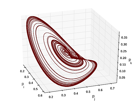
"\n",
"**Figure 14.8** A chaotic attractor for the 4-D Lotka-Volterra model projected\n",
"onto three axes."
]
},
{
"cell_type": "markdown",
"metadata": {},
"source": [
"## 14.11 Predator-Prey Chaos \n",
"\n",
"Mathematical analysis tells us that, in addition to nonlinearity, a system must\n",
"contain a minimum number of degrees of freedom before chaos will occur. For\n",
"example, for chaos to occur in a predator-prey model, there must be three or\n",
"more species present. And so to produce some real chaos we must extend our\n",
"previous treatment. Accordingly, we now extend the predator-prey model to\n",
"include four species, each with population $p_i$ competing for the same finite\n",
"set of resources. The differential equation form of the model \\[[Vano et al.(06)](BiblioLinked.html#sprott),\n",
"[Cencini et al.(10)](BiblioLinked.html#cen)\\] extends the Lotka-Volterra model (14.41) to:\n",
"\n",
"$$\\tag*{14.43}\n",
"\\frac{dp_i}{dt} = a_i p_i \\left(1-\\sum_{j=1}^4 b_{ij} p_j \\right), \\qquad i=1, 4.$$\n",
"\n",
"Here $a_i $ is a measure of the growth rate of species $i$, and $b_{ij}$\n",
"is a measure of the extent to which species $j$ consumes the resources\n",
"otherwise used by species $i$. If we require both $a_i \\geq 0$ and\n",
"$b_{ij}\\geq 0$, then all populations should remain in the range\n",
"$0\\leq p_i \\leq 1$.\n",
"\n",
"Because four species covers a very large parameter space, we suggest\n",
"that you start your exploration using the same parameters that \\[Vano et\n",
"al.(06)\\] found produces chaos:\n",
"\n",
"$$\\tag*{14.44} a_i=\\begin{pmatrix} 1\\cr\n",
" 0.72\\cr\n",
" 1.53\\cr\n",
" 1.27\\cr \\end{pmatrix},\n",
"\\qquad\n",
"b_{ij}=\\begin{pmatrix} 1& 1.09& 1.52&0\\cr\n",
" 0& 1& 0.44&1.36\\cr\n",
" 2.33& 0& 1&0.47\\cr\n",
" 1.21& 0.51& 0.35&1\\cr\\end{pmatrix}.$$\n",
"\n",
"But because chaotic systems are hyper sensitive to the exact parameter\n",
"values, you may need to modify these slightly.\n",
"\n",
"Note that the self-interactions terms $a_{ii} =1$, which is a\n",
"consequence of measuring the population of each species in units of its\n",
"individual carrying capacity. We solve (14.43) with initial conditions\n",
"corresponding to an equilibrium point at which all species coexist:\n",
"\n",
"$$\\tag*{14.45} p_i (t=0) =\\begin{pmatrix}0.3013\\cr\n",
" 0.4586\\cr\n",
" 0.1307\\cr\n",
" 0.3557\\cr\\end{pmatrix}.$$\n",
"\n",
"One way to visualize the solution to (14.43) is to make four plots of\n",
"$p_1(t), p_2(t), p_3(t),$ and $p_4(t)$ versus time. The results are\n",
"quite interesting, and we leave that as an exercise for you. A more\n",
"illuminating visualization would be to create a 4-D phase-space plot of\n",
"$[p_1(t_i), p_2(t_i), p_3(t_i), p_4(t_i)]$ for $i=1, N$, where $N$ is\n",
"the number of time steps used in your numerical solution. Even in the\n",
"presence of chaos, the geometric structure so created may have a smooth\n",
"and well-defined shape. Unfortunately, we have no way to show such a\n",
"plot, and so in its stead we must project the 4-D structure onto 2-D and\n",
"3-D axes. We show one such 3-D plot in Figure 14.8. This is a classic\n",
"type of chaotic attractor, with the 3-D structure folded over into a\n",
"nearly 2-D structure (the Rossler equation is famous for producing such\n",
"a structure).\n",
"\n",
"### 14.11.1 Exercises\n",
"\n",
"1. Solve (14.43) for the suggested parameters and initial conditions,\n",
" and make plots of $p_{1-4}(t)$ as functions of time. Comment on the\n",
" type of behavior that these plots exhibit.\n",
"\n",
"2. Construct the 4-D phase chaotic attractor formed by the solutions\n",
" of (14.43) by writing to a file the values\n",
" $[p_1(t_i), p_2(t_i), p_3(t_i), p_4(t_i)]$ where $i$ labels the\n",
" time step. In order to avoid needlessly long files, you may want to\n",
" skip a number of time steps before each file output.\n",
"\n",
" 1. Plot all possible 2-D phase space plots, that is, plots of $p_i$\n",
" *vs* $p_j$, $i \\neq j = 1-3$.\n",
"\n",
" 2. Plot all possible 3-D phase space plots, that is, plots of $p_i$\n",
" *vs* $p_j$ *vs* $p_k$.\n",
"\n",
" *Note:* you have to adjust the parameters or initial conditions\n",
" slightly to obtain truly chaotic behavior."
]
},
{
"cell_type": "markdown",
"metadata": {},
"source": [
"### 14.11.2 LVM with Prey Limit\n",
"\n",
"The initial assumption in the LVM that prey grow without limit in the absence of\n",
"predators is clearly unrealistic. As with the logistic map, we include a limit on\n",
"prey numbers that accounts for depletion of the food supply as the prey\n",
"population grows. Accordingly, we modify the constant growth rate from $a$ to\n",
"$a(1-p/K)$ so that growth vanishes when the population reaches a limit $K$,\n",
"the *carrying capacity*:\n",
"\n",
"$$\\begin{align}\n",
"\\tag*{14.46}\n",
" \\frac{dp}{dt} & = a p\\left(1-\n",
"\\frac{p}{K}\\right)-b p P,\\\\\n",
" \\frac{dP}{dt} & = \\epsilon b p P-m P \\qquad \\mbox{(LVM-II).}\\tag*{14.47}\n",
" \\end{align}$$\n",
" \n",
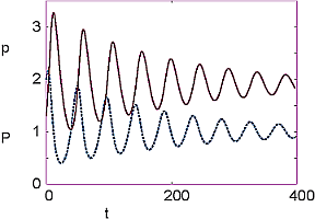
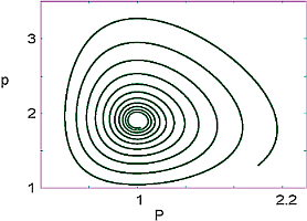
" The behavior of this model with prey limitations is\n",
"shown in Figure 14.9. We see that both populations exhibit damped\n",
"oscillations as they approach their equilibrium values, and that as\n",
"hoped for, the equilibrium populations are independent of the initial\n",
"conditions. Note how the phase space plot spirals inward to a single\n",
"close limit cycle, on which it remains, with little variation in prey\n",
"number. This is “control”, and we may use it to start a chemical-free\n",
"pest control business.\n",
"\n",
"### 14.11.3 LVM with Predation Efficiency\n",
"\n",
"An additional unrealistic assumption in the original LVM is that the\n",
"predators immediately eat all the prey with which they interact. As\n",
"anyone who has watched a cat hunt a mouse knows, predators spend some\n",
"time finding prey and also chasing, killing, eating, and digesting it\n",
"(all together called *handling*). This extra time decreases the rate\n",
"$bpP$ at which prey are eliminated. We define the *functional response*\n",
"$p_a$ as the probability of one predator finding one prey. If a single\n",
"predator spends time $t_{\\text{search}}$ searching for prey, then\n",
"\n",
"$$\\tag*{14.48} p_a = b t_{\\text{search}} p\\ \\Rightarrow\\ \n",
"t_{\\text{search}} = \\frac{p_a}{bp}.$$\n",
"\n",
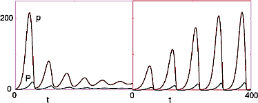
"|Fig 14.9 A|Fig 14.9 B| \n",
"|:- - -:|:- - -:| \n",
"|||\n",
"\n",
"**Figure 14.9** *A:* The Lotka-Volterra model of prey population *p(t)*\n",
"(solid curve) and predator population *P(t)* (dashed curve) versus time when a\n",
"prey population limit is included. *B:* Prey population *p* as a function\n",
"of predator population *P*.\n",
"\n",
"If we call $t_h$ the time a predator spends handling a single prey, then the\n",
"effective time a predator spends handling a prey is $p_a t_h$. Such being the\n",
"case, the total time $T$ that a predator spends finding and handling a single\n",
"prey is \n",
"\n",
"$$\\begin{align}\n",
"\\tag*{14.49}\n",
"T = t_{\\text{search}}+t_{\\text{handling}} & = \\frac{p_a}{bp}+ p_a t_h\\\\\n",
" \\Rightarrow \\quad \\frac{p_a}{T} & =\n",
"\\frac{bp}{1+bpt_h},\\tag*{14.50}\\end{align}$$ \n",
"\n",
"where $p_a/T$ is the\n",
"effective *rate* of eating prey. We see that as the number of prey\n",
"$p\\rightarrow\\infty$, the efficiency in eating them $\\rightarrow 1$. We include\n",
"this efficiency in (14.46) by modifying the rate $b$ at which a predator\n",
"eliminates prey to $b/(1+bpt_h)$:\n",
"\n",
"$$\\tag*{14.51}\n",
" \\frac{dp}{dt} =\n",
"ap\\left(1-\\frac{p}{K}\\right)-\\frac{bpP} {1+bpt_h}, \\qquad\n",
"\\mbox{(LVM-III}).$$\n",
"\n",
"To be more realistic about the predator growth, we also place a limit on\n",
"the predator carrying capacity but make it proportional to the number of\n",
"prey:\n",
"\n",
"$$\\tag*{14.52}\n",
" \\frac{dP}{dt}=mP\\left(1-\\frac{P}{kp}\\right), \\quad\n",
"\\mbox{(LVM-III}).$$\n",
"\n",
"Solutions for the extended model (14.51) and (14.52) are shown in\n",
"Figure 14.10. Observe the existence of three dynamic regimes as a\n",
"function of $b$:\n",
"\n",
"- small $b$: no oscillations, no overdamping,\n",
"\n",
"- medium $b$: damped oscillations that converge to a stable\n",
" equilibrium,\n",
"\n",
"- large $b$: limit cycle.\n",
"\n",
"The transition from equilibrium to a limit cycle is called a *phase\n",
"transition*.\n",
"\n",
"We finally have a satisfactory solution to our **problem**. Although the\n",
"prey population is not eliminated, it can be kept from getting too large\n",
"and from fluctuating widely. Nonetheless, changes in the parameters can\n",
"lead to large fluctuations or to nearly vanishing predators.\n",
"\n",
"|A|B| \n",
"|:- - -:|:- - -:| \n",
"|||\n",
"\n",
"**Figure 14.10** Lotka-Volterra model with predation efficiency and prey\n",
"limitations. From left to Bottom: overdamping, $\\textit{b} =\n",
"\\text{0.01}$; damped oscillations, $\\textit{b} = \\text{0.1}$, and limit\n",
"cycle, $\\textit{b} =\n",
"\\text{0.3}$.\n",
"\n",
"### 14.11.4 LVM Implementation and Assessment\n",
"\n",
"|*Model* | $a$ | $b$| $\\epsilon$ | $m$ | $K$ | k|\n",
"|- - -|- - -|- - -|- - -|- - -|- - -|- - -|\n",
"|LVM-I | 0.2 | 0.1 | 1 | 0.1 |0| - - -|\n",
"|LVM-II | 0.2 | 0.1 | 1 | 0.1 | 20 |- - - |\n",
"|LVM-III | 0.2 | 0.1 | - - - | 0.1 |500 | 0.2|\n",
"\n",
"1. Write a program to solve (14.51) and (14.52) using the `rk4`\n",
" algorithm and the preceeding parameter values.\n",
"\n",
"2. For each of the three models, construct\n",
"\n",
" - a time series for prey and predator populations,\n",
"\n",
" - phase space plots of predator *versus*\n",
" prey populations.\n",
"\n",
"3. **LVM-I**: Compute the equilibrium values for the prey and\n",
" predator populations. Do you think that a model in which the cycle\n",
" amplitude depends on the initial conditions can be\n",
" realistic? Explain.\n",
"\n",
"4. **LVM-II**: Calculate numerical values for the equilibrium values of\n",
" the prey and predator populations. Make a series of runs for\n",
" different values of prey carrying capacity $K$. Can you deduce how\n",
" the equilibrium populations vary with prey carrying capacity?\n",
"\n",
"5. Make a series of runs for different initial conditions for predator\n",
" and prey populations. Do the cycle amplitudes depend on the initial\n",
" conditions?\n",
"\n",
"6. **LVM-III**: Make a series of runs for different values of $b$ and\n",
" reproduce the three regimes present in Figure 14.10.\n",
"\n",
"7. Calculate the critical value for $b$ corresponding to a phase\n",
" transition between the stable equilibrium and the limit cycle."
]
},
{
"cell_type": "code",
"execution_count": null,
"metadata": {
"collapsed": false
},
"outputs": [],
"source": [
"from IPython.display import IFrame\n",
"from numpy import *\n",
"\n",
"import numpy as np\n",
"import matplotlib.pyplot as plt\n",
"\n",
"Tmin = 0.0\n",
"Tmax = 500.0 # endpoints\n",
"y = np.zeros( (2), float)\n",
"yy0=np.zeros((1002),float)\n",
"yy1=np.zeros((1002),float)\n",
"Ntimes = 1000\n",
"y[0] = 2.0\n",
"y[1] = 1.3 # initialize\n",
"h = (Tmax - Tmin)/Ntimes \n",
"t = Tmin\n",
"\n",
"def f( t, y, F): # FUNCTION of your choice here\n",
" F[0] = 0.2*y[0]*(1 - (y[0]/(20.0) )) - 0.1*y[0]*y[1] # RHS of 1st eq\n",
" F[1] = - 0.1*y[1] + 0.1*y[0]*y[1]; # RHS of 2nd eq\n",
"\t\t \n",
"def rk4(t, y, h, Neqs): # rk4 method, *DO NOT MODIFY*, instead, modify f\n",
" F = np.zeros( (Neqs), float)\n",
" ydumb = np.zeros( (Neqs), float)\n",
" k1 = np.zeros( (Neqs), float)\n",
" k2 = np.zeros( (Neqs), float)\n",
" k3 = np.zeros( (Neqs), float)\n",
" k4 = np.zeros( (Neqs), float)\n",
" f(t, y, F)\n",
" for i in range(0, Neqs):\n",
" k1[i] = h*F[i]\n",
" ydumb[i] = y[i] + k1[i]/2.\n",
" f(t + h/2., ydumb, F)\n",
" for i in range(0, Neqs):\n",
" k2[i] = h*F[i]\n",
" ydumb[i] = y[i] + k2[i]/2.\n",
" f(t + h/2., ydumb, F)\n",
" for i in range(0, Neqs):\n",
" k3[i] = h*F[i]\n",
" ydumb[i] = y[i] + k3[i]\n",
" f(t + h, ydumb, F)\n",
" for i in range(0, Neqs):\n",
" k4[i] = h*F[i]\n",
" y[i] = y[i] + (k1[i] + 2.*(k2[i] + k3[i]) + k4[i])/6.\n",
"tt=np.arange(0,Tmax+1,h)\t\t\t\t\n",
"#plt.plot(t,)\n",
"j=0\n",
"for t in np.arange(Tmin, Tmax + 1, h):\n",
" yy0[j]=y[0]\n",
" yy1[j]=y[1]\n",
" #print(j)\n",
" #funct1.plot(pos = (t, y[0]) )\n",
" #funct2.plot(pos = (t, y[1]) )\n",
" #funct3.plot(pos = (y[0], y[1]) )\n",
" #rate(60)\n",
" rk4(t, y, h, 2)\n",
" j+=1\n",
"plt.figure(0) \n",
"plt.plot(tt,yy0)\n",
"plt.title('Prey population p(green) and predator population P(blue) vs. time')\n",
"plt.ylabel('P,p')\n",
"plt.xlabel('t')\n",
"plt.plot(tt,yy1)\n",
"plt.figure(1)\n",
"plt.plot(yy0,yy1,'r')\n",
"plt.title('Predator population (P) vs prey (p) population')\n",
"plt.xlabel('p')\n",
"plt.ylabel('P')\n",
"\n",
"plt.show()"
]
},
{
"cell_type": "markdown",
"metadata": {},
"source": [
"### 14.11.5 Two Predators, One Prey (Exploration)\n",
"\n",
"1. Another version of the LVM includes the possibility that two\n",
" populations of predators $P_1$ and $P_2$ may “share” the same prey\n",
" population $p$. Investigate the behavior of a system in which the\n",
" prey population grows logistically in the absence of predators:\n",
"\n",
" $$\\begin{align}\n",
" \\frac{dp}{dt} & = ap\\left(1-\\frac{p}{K}\\right) - \\left(b_1P_1 + b_2P_2\\right)p,\\tag*{14.53} \\\\\n",
" \\frac{dP}{dt} & = \\epsilon_1b_1pP_1-m_1P_1,\\quad \\frac{dP_2}{dt} =\\epsilon_2b_2pP_2-m_2P_2.\\tag*{14.54} \\end{align}$$\n",
"\n",
"2. Use the following values for the model parameters and initial\n",
" conditions:
\n",
" \n",
" $a = 0.2$, $K = 1.7$, $b_1 = 0.1$, $b_2 = 0.2$, $m_1 = m_2 =\n",
" 0.1$, $\\epsilon_1 =1.0$, $\\epsilon_2 =2.0$, $p(0) = P_2(0) = 1.7$, and $P_1(0) = 1.0$.\n",
"\n",
"3. Determine the time dependence for each population.\n",
"\n",
"4. Vary the characteristics of the second predator and calculate the\n",
" equilibrium population for the three components.\n",
"\n",
"5. What is your answer to the question, “Can two predators that share\n",
" the same prey coexist?”\n",
"\n",
"6. The nonlinear nature of the Lotka-Volterra model can lead to chaos\n",
" and fractal behavior. Search for chaos by varying the growth rates."
]
},
{
"cell_type": "markdown",
"metadata": {},
"source": []
}
],
"metadata": {
"kernelspec": {
"display_name": "Python 2",
"language": "python",
"name": "python2"
},
"language_info": {
"codemirror_mode": {
"name": "ipython",
"version": 2
},
"file_extension": ".py",
"mimetype": "text/x-python",
"name": "python",
"nbconvert_exporter": "python",
"pygments_lexer": "ipython2",
"version": "2.7.11"
}
},
"nbformat": 4,
"nbformat_minor": 0
}