{
"cells": [
{
"cell_type": "markdown",
"metadata": {},
"source": [
"# *Chapter 16*
Fractals & Statistical Growth Models \n",
"\n",
"| | | |\n",
"|:---:|:---:|:---:|\n",
"| |[From **COMPUTATIONAL PHYSICS**, 3rd Ed, 2015](http://physics.oregonstate.edu/~rubin/Books/CPbook/index.html)
RH Landau, MJ Paez, and CC Bordeianu (deceased)
Copyrights:
[Wiley-VCH, Berlin;](http://www.wiley-vch.de/publish/en/books/ISBN3-527-41315-4/) and [Wiley & Sons, New York](http://www.wiley.com/WileyCDA/WileyTitle/productCd-3527413154.html)
R Landau, Oregon State Unv,
MJ Paez, Univ Antioquia,
C Bordeianu, Univ Bucharest, 2015.
Support by National Science Foundation.||\n",
"\n",
"**16 Fractals & Statistical Growth Models**
\n",
"[16.1 Fractional Dimension (Math)](#16.1)
\n",
"[16.2 The Sierpi´nski Gasket (Problem 1)](#16.2)
\n",
" [16.2.1 Sierpi´nski Implementation](#16.2.1)
\n",
" [16.2.2 Assessing Fractal Dimension](#16.2.2)
\n",
"[16.3 Growing Plants (Problem 2)](#16.3)
\n",
" [16.3.1 Self-Affine Connection (Theory)](#16.3.1)
\n",
" [16.3.2 Barnsley’s Fern Implementation](#16.3.2)
\n",
" [16.3.3 Self-Affinity in Trees Implementation](#16.3.3)
\n",
"[16.4 Ballistic Deposition (Problem 3)](#16.4)
\n",
" [16.4.1 Random Deposition Algorithm](#16.4.1)
\n",
"[16.5 Length of British Coastline (Problem 4)](#16.5)
\n",
" [16.5.1 Coastlines as Fractals (Model)](#16.5.1)
\n",
"[16.5.2 Box Counting Algorithm](#16.5.2)
\n",
" [16.5.3 Coastline Implementation and Exercise](#16.5.3)
\n",
"[16.6 Correlated Growth, Forests, Films (Problem 5)](#16.6)
\n",
" [16.6.1\n",
"Correlated Ballistic Deposition\n",
"Algorithm](#16.6.1)
\n",
"[16.7 Globular Cluster (Problem 6)](#16.7)
\n",
" [16.7.1 Diffusion-Limited Aggregation Algorithm](#16.7.1)
\n",
" [16.7.2 Fractal Assessment of DLA or a Pollock](#16.7.2)
\n",
"[16.8 Fractals in Bifu\n",
"rcation Plot (Problem 7)](#16.8)
\n",
"[16.9 Fractals from Cellular Automata](#16.91)
\n",
"[16.10 Perlin Noise Adds Realism](#16.10)
\n",
" [16.10.1 Ray Tracing Algorithms](#16.10.1)
\n",
"[16.11 Exercises](#16.11)
\n",
"\n",
"\n",
"\n",
"\n",
"*It is common to notice regular and eye-pleasing natural objects, such\n",
"as plants and sea shells, that do not have well-defined geometric\n",
"shapes. When analyzed mathematically with a prescription that normally\n",
"produces integers, some of these objects are found to have a dimension\n",
"that is a fractional number, and so they are called “fractals”. In this\n",
"chapter we implement simple, statistical models that grow fractals. We\n",
"emphasize the simple underlying rules, the statistical models that may\n",
"lead to such rules, and the mathematical meaning of and measurements of\n",
"self-similar objects. To the extent that these models generate\n",
"structures that look like those in nature, it is reasonable to assume\n",
"that the natural processes must be following similar rules arising from\n",
"the basic physics or biology that creates the objects. Detailed\n",
"applications of fractals can be found in the literature*\n",
"\\[[Mandelbrot(82)](BiblioLinked.html#mandel), [Armin & Shlomo(91)](BiblioLinked.html#armin), [Sander et al.(94)](BiblioLinked.html#sander), [Peitgen et\n",
"al.(94)](BiblioLinked.html#peit)\\].\n",
"\n",
"** This Chapter’s Lecture, Slide Web Links, Applets & Animations**\n",
"\n",
"| | |\n",
"|---|---|\n",
"|[All Lectures](http://physics.oregonstate.edu/~rubin/Books/CPbook/eBook/Lectures/index.html)|[](http://physics.oregonstate.edu/~rubin/Books/CPbook/eBook/Lectures/index.html)|\n",
"\n",
"| *Lecture (Flash)*| *Slides* | *Sections*|*Lecture (Flash)*| *Slides* | *Sections*| \n",
"|- - -|:- - -:|:- - -:|- - -|:- - -:|:- - -:|\n",
"|[Fractals I](http://physics.oregonstate.edu/~rubin/Books/CPbook/eBook/Lectures/Modules/Fractals_1/Fractals_1.html)|[pdf](http://physics.oregonstate.edu/~rubin/Books/CPbook/eBook/Lectures/Slides/Slides_NoAnimate_pdf/FractalsI.pdf)|13.1-.2 | [Fractals II](http://physics.oregonstate.edu/~rubin/Books/CPbook/eBook/Lectures/Modules/Fractals_2/Fractals_2.html)|[pdf](http://physics.oregonstate.edu/~rubin/Books/CPbook/eBook/Lectures/Slides/Slides_NoAnimate_pdf/FractasII_NEW.pdf)| 13.3|\n",
"|[Sierpinski Applet](http://science.oregonstate.edu/~rubin/Books/CPbook/eBook/Applets/index.html) | -|13.2 |[Fern Applet](http://science.oregonstate.edu/~rubin/Books/CPbook/eBook/Applets/index.html)| -|13.3|\n",
"|[Tree Applet](http://science.oregonstate.edu/~rubin/Books/CPbook/eBook/Applets/index.html)|-|13.3|[Film Applet](http://science.oregonstate.edu/~rubin/Books/CPbook/eBook/Applets/index.html)| -|13.4 |\n",
"|[Column](http://science.oregonstate.edu/~rubin/Books/CPbook/eBook/Applets/index.html)|-|13.6|[DLA Applet](http://science.oregonstate.edu/~rubin/Books/CPbook/eBook/Applets/index.html)| -|13.7 | \n",
"|[Ballistic Movie](http://science.oregonstate.edu/~rubin/Books/CPbook/Codes/Animations/Fractals/FractalGrowth.mp4)| 13.4|- || "
]
},
{
"cell_type": "markdown",
"metadata": {},
"source": [
"## 16.1 Fractional Dimension (Math) \n",
"\n",
"Benoit Mandelbrot, who first studied fractional-dimension figures with\n",
"supercomputers at IBM Research, gave them the name *fractals*\n",
"\\[[Mandelbrot(82)](BiblioLinked.html#mandel)\\]. Some geometric objects, such as Koch curves, are\n",
"exact fractals with the same dimension for all their parts. Other\n",
"objects, such as bifurcation curves, are statistical fractals in which\n",
"elements of apparent randomness occur and the dimension can be defined\n",
"only for each part of the object, or on the average.\n",
"\n",
"Consider an abstract object such as the density of charge within an\n",
"atom. There are an infinite number of ways to measure the “size” of this\n",
"object. For example, each moment $\\langle r^n\n",
"\\rangle$ is a measure of the size, and there is an infinite number of\n",
"such moments. Likewise, when we deal with complicated objects, there are\n",
"different definitions of dimension and each may give a somewhat\n",
"different value.\n",
"\n",
"Our first definition of the dimension $d_f$, the *Hausdorff-Besicovitch\n",
"dimension*, is based on our knowledge that a line has dimension 1, a\n",
"triangle has dimension 2, and a cube has dimension 3. It seems perfectly\n",
"reasonable to ask if there is some mathematical formula that agrees with\n",
"our experience with regular objects, yet can also be used for\n",
"determining fractional dimensions. For simplicity, let us consider\n",
"objects that have the same length $L$ on each side, as do equilateral\n",
"triangles and squares, and that have uniform density. We postulate that\n",
"the dimension of an object is determined by the dependence of its total\n",
"mass upon its length:\n",
"\n",
"$$\\tag*{16.1} M(L) \\propto L^{d_f},$$\n",
"\n",
"where the power $d_f$ is the *fractal dimension*. As you may verify,\n",
"this rule works with the 1-D, 2-D, and 3-D regular figures in our\n",
"experience, so it is a reasonable to try it elsewhere. When we apply\n",
"(16.1) to fractal objects, we end up with fractional values for $d_f$.\n",
"Actually, we will find it easier to determine the fractal dimension not\n",
"from an object’s mass, which is *extensive* (depends on size), but\n",
"rather from its density, which is *intensive*. The density is defined as\n",
"mass/length for a linear object, as mass/area for a planar object, and\n",
"as mass/volume for a solid object. That being the case, for a planar\n",
"object we hypothesize that\n",
"\n",
"$$\\tag*{16.2}\n",
"\\rho =\\frac{M(L)}{\\mbox{area}} \\propto \\frac{L^{d_f}}{L^2}\\propto\n",
"L^{d_f-2}.$$\n",
"\n",
"| | |\n",
"|:- - -:|:- - -:| \n",
"| ||\n",
"\n",
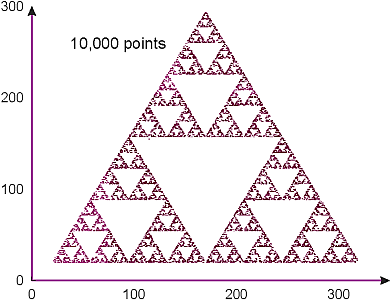
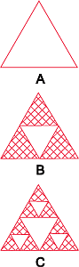
"**Figure 16.1** *A:* A statistical fractal Sierpiński gasket containing 10,000\n",
"points. Note the self-similarity at different scales. *B:* A geometric\n",
"Sierpiński gasket constructed by successively connecting the midpoints of the\n",
"sides of each equilateral triangle. The first three steps in the process are labeled\n",
"as A, B, C."
]
},
{
"cell_type": "markdown",
"metadata": {},
"source": [
"## 16.2 The Sierpiński Gasket (Problem 1)\n",
"\n",
"| | |\n",
"|---|---|\n",
"||[Sierpinski Applet](http://science.oregonstate.edu/~rubin/Books/CPbook/eBook/Applets/index.html)\n",
"\n",
"To generate our first fractal (Figure 16.1), we play a game of chance in\n",
"which we place dots at points picked randomly within a triangle \\[[Bunde\n",
"& Havlin(91)](BiblioLinked.html#bunde)\\]. try out in the margins now).\n",
"\n",
"1. Draw an equilateral triangle with vertices and coordinates:\n",
"\n",
" $$\\tag*{16.3}\n",
" \\mbox{vertex } 1\\colon (a_1,b_1);\\enspace \\mbox{vertex } 2\\colon\n",
" (a_2,b_2);\\enspace \\mbox{vertex } 3\\colon (a_3,b_3).$$\n",
"\n",
"2. Place a dot at an arbitrary point $P=(x_0,y_0)$ within\n",
" this triangle.\n",
"\n",
"3. Find the next point by selecting randomly the integer $1$, $2$, or\n",
" $3$:\n",
"\n",
" - If $1$, place a dot halfway between $P$ and vertex 1.\n",
"\n",
" - If $2$, place a dot halfway between $P$ and vertex 2.\n",
"\n",
" - If $3$, place a dot halfway between $P$ and vertex 3.\n",
"\n",
"4. Repeat the process using the last dot as the new $P$.\n",
"\n",
"Mathematically, the coordinates of successive points are given by the formulas\n",
"\n",
"$$\\tag*{16.4}\n",
" (x_{k+1},y_{k+1})=\\frac{(x_k,y_k)+ (a_n,b_n)}{2}, \\quad n =\n",
"\\mbox{integer} (1 + 3 r_i),$$\n",
"\n",
"where $r_i$ is a random number between $0$ and $1$ and where the\n",
"*integer* function outputs the closest integer smaller than or equal to\n",
"the argument. After 15,000 points, you should obtain a collection of\n",
"dots like those on the left in Figure 16.1.\n",
"\n",
"### 16.2.1 Sierpiński Implementation\n",
"\n",
"Write a program to produce a Sierpiński gasket. Determine empirically\n",
"the fractal dimension of your figure. Assume that each dot has mass $1$\n",
"and that $\\rho=C L^{\\alpha}$. (You can have the computer do the counting\n",
"by defining an array *box* of all $0$ values and then change a $0$ to a\n",
"$1$ when a dot is placed there.)"
]
},
{
"cell_type": "markdown",
"metadata": {},
"source": [
"### 16.2.2 Assessing Fractal Dimension\n",
"\n",
"The topology in Figure 16.1 was first analyzed by the Polish\n",
"mathematician Sierpiński. Observe that there is the same structure in a\n",
"small region as there is in the entire figure. In other words, if the\n",
"figure had infinite resolution, any part of the figure could be scaled\n",
"up in size and would be similar to the whole. This property is called\n",
"*self-similarity*.\n",
"\n",
"We construct a non-statistical form of the Sierpiński gasket by removing\n",
"an inverted equilateral triangle from the center of all filled\n",
"equilateral triangles to create the next figure (Figure 16.1 right). We\n",
"then repeat the process ad infinitum, scaling up the triangles so each\n",
"one has side $r=1$ after each step. To see what is unusual about this\n",
"type of object, we look at how its density (mass/area) changes with\n",
"size, and then apply (16.2) to determine its fractal dimension. Assume\n",
"that each triangle has mass $m$ and assign unit density to the single\n",
"triangle:\n",
"\n",
"$$\\tag*{16.5}\n",
" \\rho(L=r) \\propto\\frac{M}{r^2} = \\frac{m}{r^2} = \\rho_0 \\qquad\n",
"\\mbox{(Figure 16.1A)}$$\n",
"\n",
"Next, for the equilateral triangle with side $L=2$, the density is\n",
"\n",
"$$\\tag*{16.6}\n",
"\\qquad \\rho(L=2r) \\propto\\frac{(M=3m)}{(2r)^2} =\\frac{3}{4}mr^2 =\n",
"\\frac{3}{4} \\rho_0 \\qquad\n",
"\\mbox{(Figure 16.1B)}$$\n",
"\n",
"We see that the extra white space in Figure 16.1B leads to a density\n",
"that is $\\frac{3}{4}$ that of the previous stage. For the structure in\n",
"Figure 16.1C, we obtain\n",
"\n",
"$$\\tag*{16.8}\n",
"\\qquad\\rho(L=4r) \\propto\\frac{(M=9m)}{(4r)^2} = \\frac{9}{16}\n",
"\\frac{m}{r^2} = \\left(\\frac{3}{4}\\right)^2 \\rho_0. \\qquad\n",
"\\mbox{(Figure 16.1C)}$$\n",
"\n",
"We see that as we continue the construction process, the density of each\n",
"new structure is $\\frac{3}{4}$ that of the previous one. Interesting.\n",
"Yet in (16.2) we derived that\n",
"\n",
"$$\\tag*{16.9} {\\rho \\propto C L^{d_f-2}}.$$\n",
"\n",
"Equation (16.9) implies that a plot of the logarithm of the density\n",
"$\\rho$ *versus* the logarithm of the length $L$ for successive\n",
"structures yields a straight line of slope\n",
"\n",
"$$d_f-2 = \\frac{\\Delta \\log\\rho}{\\Delta \\log L}.$$\n",
"\n",
"As applied to our problem,\n",
"\n",
"$$\\tag*{16.10} d_f = 2+ \\frac{\\Delta \\log\\rho(L)}{\\Delta \\log L}= 2+ \\frac{\\log\n",
"1-\\log \\frac{3}{4}}{log 1 -\\log 2} \\simeq 1.58496.$$\n",
"\n",
"As is evident in Figure 16.1, as the gasket grows larger (and\n",
"consequently more massive), it contains more open space. So despite the\n",
"fact that its mass approaches infinity as $L\\rightarrow\\infty$, its\n",
"density approaches zero! And because a 2-D figure like a solid triangle\n",
"has a constant density as its length increases, a 2-D figure has a slope\n",
"equal to $0$. Because the Sierpiński gasket has a slope $d_f-2 \\simeq\n",
"-0.41504$, it fills space to a lesser extent than a 2-D object but more\n",
"so than a 1-D object; it is a fractal with dimension 1.6."
]
},
{
"cell_type": "markdown",
"metadata": {},
"source": [
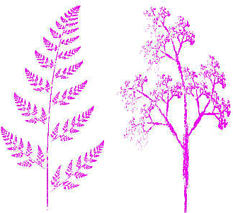
"## 16.3 Growing Plants (Problem 2) \n",
"\n",
"It seems paradoxical that natural processes subject to chance can\n",
"produce objects of high regularity and symmetry. For example, it is hard\n",
"to believe that something as beautiful and graceful as a fern\n",
"(Figure 16.2 left) has random elements in it. Nonetheless, there is a\n",
"clue here in that much of the fern’s beauty arises from the similarity\n",
"of each part to the whole (self-similarity), with different ferns\n",
"similar but not identical to each other. These are characteristics of\n",
"fractals. Your **problem** is to discover if a simple algorithm\n",
"including some randomness can draw regular ferns. If the algorithm\n",
"produces objects that resemble ferns, then presumably you have uncovered\n",
"mathematics similar to that responsible for the shapes of ferns.\n",
"\n",
"\n",
"\n",
"**Figure 16.2** *Top:* A fractal fern\n",
"generated by 30,000 iterations of the algorithm ( 16.14).\n",
"Enlarging this fern shows that each frond with a similar structure.\n",
"*Bottom:* A fractal tree created with the simple algorithm (16.7).\n",
"\n",
"### 16.3.1 Self-Affine Connection ( Theory)\n",
"\n",
"In (16.4), which defines mathematically how a Sierpiński gasket is\n",
"constructed, a *scaling factor* of $\\frac{1}{2}$ is part of the relation\n",
"of one point to the next. A more general transformation of a point\n",
"$P=(x,y)$ into another point $P'=(x',y')$ via *scaling* is\n",
"\n",
"$$\\tag*{16.11} (x', y')=s(x, y) =(sx,sy) \\quad\\mbox{(scaling).}$$\n",
"\n",
"If the scale factor $s>0$, an amplification occurs, whereas if $s<0$, a\n",
"reduction occurs. In our definition (16.4) of the Sierpiński gasket, we\n",
"also added in a constant $a_n$. This is a *translation operation*, which\n",
"has the general form\n",
"\n",
"$$\\tag*{16.12} (x', y') =(x,y) +(a_x, a_y)\\quad\\mbox{(translation).}$$\n",
"\n",
"Another operation, not used in the Sierpiński gasket, is a *rotation* by\n",
"angle $\\theta$:\n",
"\n",
"$$\\tag*{16.13} x'=x \\cos\\theta -y\\sin\\theta, \\quad y'=x \\sin \\theta+y \\cos\n",
"\\theta \\quad \\mbox{(rotation).}$$\n",
"\n",
"The entire set of transformations, scalings, rotations, and translations\n",
"defines an *affine transformation* (affine denotes a close relation\n",
"between successive points). The transformation is still considered\n",
"affine even if it is a more general linear transformation with the\n",
"coefficients not all related by a single $\\theta$ (in that case, we can\n",
"have contractions and reflections). What is important is that the object\n",
"created with these rules turns out to be self-similar; each step leads\n",
"to new parts of the object that bear the same relation to the ancestor\n",
"parts as the ancestors did to theirs. This is what makes the object look\n",
"similar at all scales.\n",
"\n",
"### 16.3.2 Barnsley’s Fern Implementation\n",
"\n",
"We obtain a Barnsley’s fern \\[[Barnsley & Hurd(92)](BiblioLinked.html#barns)\\] by extending the\n",
"dots game to one in which new points are selected using an affine\n",
"connection with some elements of chance mixed in:\n",
"\n",
"$$\\tag*{16.14} \n",
"(x,y)_{n+1}=\\begin{cases}\n",
" (0.5,0.27y_n),& \\mbox{with 2% probability},\\\\\n",
" (-0.139x_n+0.263y_n+0.57 & \\\\\n",
" \\ \\ 0.246x_n+0.224y_n-0.036), &\\mbox{with 15% probability},\\\\\n",
" (0.17x_n-0.215y_n+0.408 & \\\\\n",
"\\ \\ 0.222x_n+0.176y_n+0.0893),&\\mbox{with 13% probability}, \\\\\n",
" (0.781x_n+0.034y_n+0.1075 \\\\\n",
"\\ \\ -0.032x_n+0.739y_n+0.27), & \\mbox{with 70% probability.}\n",
" \\end{cases}$$\n",
"\n",
"To select a transformation with probability ${\\cal P}$, we select a\n",
"uniform random number $0 \\leq r \\leq 1$ and perform the transformation\n",
"if $r$ is in a range proportional to ${\\cal\n",
"P}$:\n",
"\n",
"$$\\tag*{16.15}\n",
"\\mbox{$\\cal P$} =\n",
" \\begin{cases}\n",
" 2 \\%,& r \\leq 0.02 , \\\\\n",
"15 \\%,& 0.02 \\leq r \\leq 0.17,\\\\\n",
"13 \\%,& 0.17 \\leq r \\leq 0.3, \\\\ 70 \\%, & 0.3 \\leq r\\leq 1.\n",
"\\end{cases}$$\n",
"\n",
"The rules (16.14) and (16.15) can be combined into one:\n",
"\n",
"$$\\tag*{16.16} \n",
"(x,y)_{n+1}= \n",
" \\begin{cases}\n",
"(0.5,0.27y_n),& r< 0.02, \\\\\n",
" (-0.139x_n+0.263y_n+0.57& \\\\\n",
" \\ \\ 0.246x_n+0.224y_n-0.036),& 0.02 \\leq r \\leq 0.17, \\\\\n",
" (0.17x_n-0.215y_n+0.408 & \\\\ \\ \\ 0.222x_n+0.176y_n+0.0893),&\n",
" 0.17 \\leq r \\leq 0.3, \\\\\n",
" (0.781x_n+0.034y_n+0.1075,\\\\ \\ \\ -0.032x_n+0.739y_n+0.27), &\n",
" 0.3 \\leq r \\leq 1 .\n",
" \\end{cases}$$\n",
"\n",
"Although (16.14) makes the basic idea clearer, (16.16) is easier to\n",
"program, which we do in Listing 16.1.\n",
"\n",
"The starting point in Barnsley’s fern (Figure 16.2) is\n",
"$(x_1,y_1)=(0.5,0.0)$, and the points are generated by repeated\n",
"iterations. An important property of this fern is that it is not\n",
"completely self-similar, as you can see by noting how different the\n",
"stems and the fronds are. Nevertheless, the stem can be viewed as a\n",
"compressed copy of a frond, and the fractal obtained with (16.14) is\n",
"still *self-affine*, yet with a dimension that varies from part to part\n",
"in the fern.\n",
"\n",
"[**Listing 16.1 Fern3D.py**](http://www.science.oregonstate.edu/~rubin/Books/CPbook/Codes/PythonCodes/Fractals/Fern3D.py) simulates the growth of ferns in 3-D.\n",
"\n",
"| | |\n",
"|---|---|\n",
"||[Fractal Growth Movie](http://science.oregonstate.edu/~rubin/Books/CPbook/eBook/Movies/FractalGrowth.mp4)|"
]
},
{
"cell_type": "code",
"execution_count": 1,
"metadata": {
"collapsed": true
},
"outputs": [],
"source": [
"### Fern.py, Notebook Version"
]
},
{
"cell_type": "code",
"execution_count": 2,
"metadata": {
"collapsed": false
},
"outputs": [
{
"ename": "ImportError",
"evalue": "No module named ivisual",
"output_type": "error",
"traceback": [
"\u001b[1;31m---------------------------------------------------------------------------\u001b[0m",
"\u001b[1;31mImportError\u001b[0m Traceback (most recent call last)",
"\u001b[1;32m\u001b[0m in \u001b[0;36m\u001b[1;34m()\u001b[0m\n\u001b[0;32m 2\u001b[0m \u001b[1;33m\u001b[0m\u001b[0m\n\u001b[0;32m 3\u001b[0m \u001b[1;32mfrom\u001b[0m \u001b[0m__future__\u001b[0m \u001b[1;32mimport\u001b[0m \u001b[0mdivision\u001b[0m\u001b[1;33m,\u001b[0m\u001b[0mprint_function\u001b[0m\u001b[1;33m\u001b[0m\u001b[0m\n\u001b[1;32m----> 4\u001b[1;33m \u001b[1;32mfrom\u001b[0m \u001b[0mivisual\u001b[0m \u001b[1;32mimport\u001b[0m \u001b[1;33m*\u001b[0m\u001b[1;33m\u001b[0m\u001b[0m\n\u001b[0m\u001b[0;32m 5\u001b[0m \u001b[1;32mfrom\u001b[0m \u001b[0mIPython\u001b[0m\u001b[1;33m.\u001b[0m\u001b[0mdisplay\u001b[0m \u001b[1;32mimport\u001b[0m \u001b[0mIFrame\u001b[0m\u001b[1;33m\u001b[0m\u001b[0m\n\u001b[0;32m 6\u001b[0m \u001b[1;32mimport\u001b[0m \u001b[0mrandom\u001b[0m\u001b[1;33m\u001b[0m\u001b[0m\n",
"\u001b[1;31mImportError\u001b[0m: No module named ivisual"
]
}
],
"source": [
"### Fern.py, Notebook Version\n",
"\n",
"from __future__ import division,print_function\n",
"from ivisual import *\n",
"from IPython.display import IFrame\n",
"import random\n",
"from numpy import *\n",
"\n",
"#pts = points(color=color.green, size=0.01)\n",
"scene=canvas(title=\"Fern 3D\")\n",
"scene.width=400\n",
"scene.height=400\n",
"#scene.forward=(-3,0,-1)\n",
"scene.range=10 #means: -10< x,y,z<10,\n",
"imax = 4000 #points to draw\n",
"i = 0\n",
"x = 0.5 #initial x coord.\n",
"y = 0.0 #initial y coord.\n",
"z = -0.2\n",
"xn = 0.0\n",
"yn = 0.0\n",
"for i in range(1,imax):\n",
" \n",
" r = random.random(); # random number\n",
" if ( r <= 0.1): #10% probability\n",
" xn = 0.0\n",
" yn = 0.18*y\n",
" zn= 0.0\n",
" \n",
" \n",
" elif ( r > 0.1 and r <= 0.7): #60% probability\n",
" xn = 0.85 * x\n",
" yn = 0.85 * y + 0.1 * z + 1.6\n",
" zn=-0.1*y + 0.85*z\n",
" #print xn,yn,zn\n",
" elif ( r > 0.7 and r <= 0.8): #15 % probability\n",
" xn = 0.2 * x - 0.2* y \n",
" yn = 0.2 * x + 0.2 * y + 0.8\n",
" zn= 0.3*z\n",
" else:\n",
" xn = -0.2 * x +0.2 *y #15% probability\n",
" yn = 0.2 * x +0.2 *y + 0.8\n",
" zn=0.3*z\n",
" x=xn #new positions are the old ones\n",
" y=yn\n",
" z=zn\n",
" xc=4.0*x #linear transformations for plotting\n",
" yc=2.0*y-7 \n",
" zc=z\n",
" genpts=points(pos=[(xc,yc,zc)],color=(0,1,0),size=1.8)"
]
},
{
"cell_type": "markdown",
"metadata": {},
"source": [
"### 16.3.2 Self-Affinity in Trees Implementation\n",
"\n",
"Now that you know how to grow ferns, look around and notice the regularity in\n",
"trees (such as in Figure 16.2 right).Can it be that this also arises from a\n",
"self-affine structure? Write a program, similar to the one for the fern, starting at\n",
"$(x_1,y_1) = (0.5,0.0)$ and iterating the following self-affine transformation:\n",
"\n",
"$$\\tag*{16.17} \n",
"(x_{n+1},y_{n+1}) \n",
"=\\begin{cases} (0.05 x_n,0.6 y_n), &\n",
"\\mbox{10% probability},\\\\\n",
"(0.05x_n, -0.5y_n+1.0), & \\mbox{10%\n",
"probability},\\\\\n",
"(0.46 x_n -0.15 y_n,0.39 x_n+0.38 y_n + 0.6), &\n",
" \\mbox{20% probability},\\\\\n",
"(0.47 x_n-0.15 y_n,0.17 x_n +0.42 y_n+1.1), &\n",
" \\mbox{20% probability},\\\\\n",
"(0.43 x_n+0.28 y_n,-0.25 x_n+0.45 y_n+1.0), &\n",
" \\mbox{20% probability},\\\\\n",
" (0.42 x_n+0.26 y_n,-0.35 x_n + 0.31 y_n+0.7), &\n",
" \\mbox{20% probability}.\n",
" \\end{cases}$$"
]
},
{
"cell_type": "markdown",
"metadata": {},
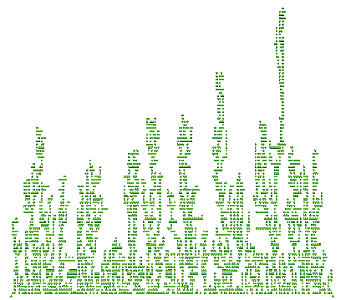
"source": [
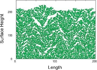
"## 16.4 Ballistic Deposition (Problem 3) \n",
"\n",
"There are a number of physical and manufacturing processes in which\n",
"particles are deposited on a surface and form a film. Because the\n",
"particles are evaporated from a hot filament, there is randomness in the\n",
"emission process yet the produced films turn out to have well-defined,\n",
"regular structures. Again we suspect fractals. Your **problem** is to\n",
"develop a model that simulates this growth process and compare your\n",
"produced structures to those observed.\n",
"\n",
"\n",
"\n",
"**Figure 16.3** A simulation of the ballistic deposition of 20,000 particles onto\n",
"a substrate of length 200. The vertical height increases in proportion to the\n",
"length of deposition time, with the top being the final surface.\n",
"\n",
"### 16.4.1 Random Deposition Algorithm\n",
"\n",
"The idea of simulating random depositions was first reported in\n",
"\\[[Vold(59)](BiblioLinked.html#vold)\\], which includes tables of random numbers used to simulate\n",
"the sedimentation of moist spheres in hydrocarbons. We shall examine a\n",
"method of simulation that results in the deposition shown in Figure 16.3\n",
"\\[[Family & Vicsek(85)](BiblioLinked.html#fer)\\].\n",
"\n",
"Consider particles falling onto and sticking to a horizontal line of\n",
"length $L$ composed of 200 deposition sites. All particles start from\n",
"the same height, but to simulate their different velocities, we assume\n",
"they start at random distances from the left side of the line. The\n",
"simulation consists of generating uniform random sites between $0$ and\n",
"$L$, and having a particle stick to the site on which it lands. Because\n",
"a realistic situation may have columns of aggregates of different\n",
"heights, the particle may be stopped before it makes it to the line, or\n",
"it may bounce around until it falls into a hole. We therefore assume\n",
"that if the column height at which the particle lands is greater than\n",
"that of both its neighbors, it will add to that height. If the particle\n",
"lands in a hole, or if there is an adjacent hole, it will fill up the\n",
"hole. We speed up the simulation by setting the height of the hole equal\n",
"to the maximum of its neighbors:\n",
"\n",
"1. Choose a random site $r$.\n",
"\n",
"2. Let the array $h_r$ be the height of the column at site $r$.\n",
"\n",
"3. Make the decision:\n",
"\n",
" $$\\tag*{16.18}\n",
" h_r =\\begin{cases}\n",
" h_r+1, & \\mbox{if } h_r \\geq h_{r-1}, \\ \\ h_r >h_{r+1},\\\\\n",
" \\mbox{max}[h_{r-1}, h_{r+1}], &\\mbox{if}\\ h_r< h_{r-1}, \\ \\ h_r<\n",
" h_{r+1}.\n",
" \\end{cases}$$\n",
"\n",
"\n",
"Our simulation [Coastline.py](http://www.science.oregonstate.edu/~rubin/Books/CPbook/Codes/PythonCodes/Fractals/Coastline.py) simulates the growth of ferns in 3-D with the essential loop:\n",
"\n",
" spot = int(random)\n",
" if (spot == 0)\n",
" if ( coast[spot] < coast[spot+1] )\n",
" coast[spot] = coast[spot+1];\n",
" else coast[spot]++;\n",
" else if (spot == coast.length - 1)\n",
" if (coast[spot] < coast[spot-1]) coast[spot] = coast[spot-1];\n",
" else coast[spot]++;\n",
" else if ( coast[spot] coast[spot+1] ) coast[spot] = coast[spot-1];\n",
" else coast[spot] = coast[spot+1];\n",
" else coast[spot]++;\n",
"\n",
"\n",
"The results of this type of simulation show several empty regions\n",
"scattered throughout the line (Figure 16.3), which is an indication of\n",
"the statistical nature of the process while the film is growing.\n",
"Simulations by Fereydoon reproduced the experimental observation that\n",
"the average height increases linearly with time and produced fractal\n",
"surfaces. (You will be asked to determine the fractal dimension of a\n",
"similar surface as an exercise.)\n",
"\n",
"**Exercise:** Extend the simulation of random deposition to two\n",
"dimensions, so rather than making a line of particles we now deposit an\n",
"entire surface."
]
},
{
"cell_type": "markdown",
"metadata": {},
"source": [
"## 16.5 Length of British Coastline (Problem 4) \n",
"\n",
"In 1967 Mandelbrot asked a classic question, “How long is the coast of\n",
"Britain?” \\[[Mandelbrot(67)](BiblioLinked.html#coast)\\]. If Britain had the shape of Colorado or\n",
"Wyoming, both of which have straight-line boundaries, its perimeter\n",
"would be a curve of dimension $1$ with finite length. However,\n",
"coastlines are geographic not geometric curves, with each portion of the\n",
"coast sometimes appearing self-similar to the entire coast. If the\n",
"perimeter of the coast is in fact a fractal, then its length is either\n",
"infinite or meaningless. Mandelbrot deduced the dimension of the west\n",
"coast of Britain to be $d_f=1.25$, which implies infinite length. In\n",
"your **problem** we ask you to determine the dimension of the perimeter\n",
"of one of our fractal simulations.\n",
"\n",
"|A|B| \n",
"|:- - -:|:- - -:| \n",
"|| |\n",
"\n",
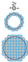
"**Figure 16.4** *A:* Example of the use of “box” counting to determine\n",
"fractal dimension. Here the “boxes” are circles and the perimeter is being\n",
"covered. The fractal dimension can be deduced by recording the number of box\n",
"of different scale needed to cover the figures. *B:* Example of the use of\n",
"“box” counting to determine fractal dimension.Here an entire figure is being\n",
"covered, and on the right a “coastline” is being covered by boxes of two\n",
"different sizes (scales). The fractal dimension can be deduced by recording the\n",
"number of box of different scale needed to cover the figures.\n",
"\n",
"### 16.5.1 Coastlines as Fractals (Model)\n",
"\n",
"The length of the coastline of an island is the perimeter of that\n",
"island. While the concept of perimeter is clear for regular geometric\n",
"figures, some thought is required to give it meaning for an object that\n",
"may be infinitely self-similar. Let us assume that a map maker has a\n",
"ruler of length $r$. If she walks along the coastline and counts the\n",
"number of times $N$ that she must place the ruler down in order to\n",
"*cover* the coastline, she will obtain a value for the length $L$ of the\n",
"coast as $Nr$. Imagine now that the map maker keeps repeating her walk\n",
"with smaller and smaller rulers. If the coast was a geometric figure or\n",
"a *rectifiable curve*, at some point the length $L$ would become\n",
"essentially independent of $r$ and would approach a constant.\n",
"Nonetheless, as discovered empirically by \\[[Richardson(61)](BiblioLinked.html#Rich61)\\] for natural\n",
"coastlines such as those of South Africa and Britain, the perimeter\n",
"appears to be an unusual function of $r$:\n",
"\n",
"$$\\tag*{16.19} L(r) = M r^{1-d_f} ,$$\n",
"\n",
"where $M$ and $d_f$ are empirical constants. For a geometric figure or\n",
"for Colorado, $d_f=1$ and the length approaches a constant as\n",
"$r\\rightarrow 0$. Yet for a fractal with $d_f>1$, the perimeter\n",
"$L\\rightarrow \\infty$ as $r\\rightarrow 0$. This means that as a\n",
"consequence of self-similarity, fractals may be of finite size but have\n",
"infinite perimeters. Physically, at some point there may be no more\n",
"details to discern as $r\\rightarrow 0$ (say, at the quantum or Compton\n",
"size limit), and so the limit may not be meaningful.\n",
"\n",
"### 16.5.2 Box Counting Algorithm\n",
"\n",
"Consider a line of length $L$ broken up into segments of length $r$ (Figure 16.4\n",
"left). The number of segments or “boxes” needed to cover the line is related to\n",
"the size $r$ of the box by \n",
"\n",
"$$\\begin{align}\n",
"\\tag*{16.20}\n",
" N(r) = \\frac{L}{r} = \\frac{C}{r},\\end{align}$$ \n",
" \n",
"where $C$ is a\n",
"constant. A proposed definition of fractional dimension is the power of\n",
"$r$ in this expression as $r\\rightarrow\n",
"0$. In our example, it tells us that the line has dimension $d_f=1.$ If\n",
"we now ask how many little circles of radius $r$ it would take to\n",
"*cover* or fill a circle of area $A$ (Figure 16.4 middle), we will find\n",
"that\n",
"\n",
"$$\\tag*{16.21} N(r) = \\lim_{r\\rightarrow 0} \\frac{A } { \\pi r^2}\n",
"\\ \\Rightarrow\\ d_f=2,$$\n",
"\n",
"as expected. Likewise, counting the number of little spheres or cubes that can\n",
"be packed within a large sphere tells us that a sphere has dimension $d_f=3.$ In\n",
"general, if it takes $N$ little spheres or cubes of side $r\\rightarrow 0$ to cover\n",
"some object, then the fractal dimension $d_f$ can be deduced as\n",
"\n",
"$$\\begin{align}\n",
"\\tag*{16.22}\n",
"N(r) & = C\\left(\\frac{1}{r}\\right)^{d_f} = C' s^{d_f} &\\quad (\\mbox{as}\\\n",
"r\\rightarrow 0),\\\\\n",
"\\log N(r) & = \\log C - d_f \\log (r) \\quad& (\\mbox{as}\\\n",
"r\\rightarrow 0),\\tag*{16.23}\\\\\n",
"\\Rightarrow \\quad d_f & = -\\lim_{r\\rightarrow 0} \\frac{\\Delta\n",
"\\log N(r)}{\\Delta \\log r}. \\tag*{16.24}\\end{align}$$ \n",
"\n",
"Here\n",
"$s \\propto 1/r$ is called the *scale* in geography, so $r\\rightarrow 0$\n",
"corresponds to an infinite scale. To illustrate, you may be familiar\n",
"with the low scale on a map being 10,000 m to a centimeter, while the\n",
"high scale is 100 m to a centimeter. If we want the map to show small\n",
"details (sizes), we need a map of high scale.\n",
"\n",
"We will use box counting to determine the dimension of a perimeter, not\n",
"of an entire figure. Once we have a value for $d_f$, we can determine a\n",
"value for the length of the perimeter via (16.19). (If you cannot wait\n",
"to see box counting in action, in the auxiliary online files you will\n",
"find an applet `Jfracdim` that goes through all the steps of box\n",
"counting before your eyes and even plots the results.)\n",
"\n",
"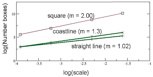\n",
"\n",
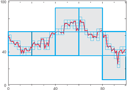
" **Figure 16.5** Fractal dimensions of a line,\n",
"box, and coastline determined by box counting. The slope at vanishingly\n",
"small scale determines the dimension.\n",
"\n",
"### 16.5.3 Coastline Implementation and Exercise\n",
"\n",
"Rather than ruin our eyes using a geographic map, we use a mathematical\n",
"one, specifically, the top portion of Figure 16.3 that maybe looks like\n",
"a natural coastline. Determine $d_f$ by covering this figure, or one you\n",
"have generated, with a semitransparent piece of graph paper \\[*Note:*\n",
"Yes, we are suggesting a painfully analog technique based on the theory\n",
"that trauma leaves a lasting impression. If you prefer, you can store\n",
"your output as a matrix of 1 and 0 values and let the computer do the\n",
"counting, but this will take more of your time!\\], and counting the\n",
"number of boxes containing any part of the coastline (Figures 16.4 and\n",
"16.5).\n",
"\n",
"1. Print your coastline graph with the same physical scale (*aspect\n",
" ratio*) for the vertical and horizontal axes. This is required\n",
" because the graph paper you will use for box counting has square\n",
" boxes and so you want your graph to also have the same vertical and\n",
" horizontal scales. Place a piece of graph paper over your printout\n",
" and look though the graph paper at your coastline. If you do not\n",
" have a piece of graph paper available, or if you are unable to\n",
" obtain a printout with the same aspect ratio for the horizontal and\n",
" vertical axes, add a series of closely spaced horizontal and\n",
" vertical lines to your coastline printout and use these lines as\n",
" your graph paper. (Box counting should still be accurate if both\n",
" your coastline and your graph paper are have the same\n",
" aspect ratios.)\n",
"\n",
"2. The vertical height in our printout was $17$ cm, and the largest\n",
" division on our graph paper was $1$ cm. This sets the scale of the\n",
" graph as 1:17, or $s=17$ for the largest divisions (lowest scale).\n",
" Measure the vertical height of your fractal, compare it to the size\n",
" of the biggest boxes on your “piece” of graph paper, and thus\n",
" determine your lowest scale.\n",
"\n",
"3. With our largest boxes of $1 \\mbox{cm} \\times 1 \\mbox{cm}$, we found\n",
" that the coastline passed through $N=24$ large boxes, that is, that\n",
" 24 large boxes covered the coastline at $s=17$. Determine how many\n",
" of the largest boxes (lowest scale) are needed to cover\n",
" your coastline.\n",
"\n",
"4. With our next smaller boxes of $0.5 \\mbox{cm} \\times\n",
" 0.5 \\mbox{cm}$, we found that 51 boxes covered the coastline at a\n",
" scale of $s=34$. Determine how many of the midsize boxes\n",
" (midrange scale) are needed to cover your coastline.\n",
"\n",
"5. With our smallest boxes of $1 \\mbox{mm} \\times 1 \\mbox{mm}$, we\n",
" found that 406 boxes covered the coastline at a scale of $s=170$.\n",
" Determine how many of the smallest boxes (highest scale) are needed\n",
" to cover your coastline.\n",
"\n",
"6. Equation (16.24) tells us that as the box sizes get progressively\n",
" smaller, we have \n",
" \n",
" $$\\begin{align}\n",
" \\log N &\\simeq \\log A + d_f \\log s, \\\\*[1ex]\n",
" \\Rightarrow \\quad d_f & \\simeq \\frac{\\Delta \\log N}{\\Delta \\log\n",
" s} =\\frac{\\log N_2 - \\log N_1}{\\log s_2-\\log s_1} =\n",
" \\frac{\\log(N_2/N_1)}{\\log (s_2/s_1)}.\n",
" \\end{align}$$ \n",
" \n",
" Clearly, only the relative scales matter because\n",
" the proportionality constants cancel out in the ratio. A plot of\n",
" $\\log N$ *versus* $\\log\n",
" s$ should yield a straight line. In our example we found a slope of\n",
" $d_f=1.23$. Determine the slope and thus the fractal dimension for\n",
" your coastline. Although only two points are needed to determine the\n",
" slope, use your lowest scale point as an important check. (Because\n",
" the fractal dimension is defined as a limit for infinitesimal box\n",
" sizes, the highest scale points are more significant.)\n",
"\n",
"7. As given by (16.19), the perimeter of the coastline\n",
"\n",
" $$\\tag*{16.25}\n",
" L\\propto s^{1.23-1} = s^{0.23}.$$\n",
"\n",
" If we keep making the boxes smaller and smaller so that we are\n",
" looking at the coastline at higher and higher scale *and* if the\n",
" coastline is self-similar at all levels, then the scale $s$ will\n",
" keep getting larger and larger with no limits (or at least until we\n",
" get down to some quantum limits). This means\n",
"\n",
" $$\\tag*{16.26}\n",
" L \\propto \\lim_{s\\rightarrow \\infty}s^{0.23} = \\infty.$$\n",
"\n",
" Does your fractal imply an infinite coastline? Does it make sense\n",
" that a small island like Britain, which you can walk around, has an\n",
" infinite perimeter?"
]
},
{
"cell_type": "markdown",
"metadata": {},
"source": [
"## 16.6 Correlated Growth, Forests, Films (Problem 5) \n",
"\n",
"It is an empirical fact that in nature there is increased likelihood\n",
"that a plant will grow if there is another one nearby (Figure 16.1A).\n",
"This *correlation* is also valid for the simulation of surface films, as\n",
"in the previous algorithm. Your **problem** is to include correlations\n",
"in the surface simulation.\n",
"\n",
"### 16.6.1 Correlated Ballistic Deposition\n",
"\n",
"A variation of the ballistic deposition algorithm, known as the *correlated\n",
"ballistic deposition*, simulates mineral deposition onto substrates on which\n",
"dendrites form \\[[Tait et al.(90)](BiblioLinked.html#tait)\\]. In Listing 16.2 we extend the previous\n",
"algorithm to include the likelihood that a freshly deposited particle will attract\n",
"another particle. We assume that the probability of sticking ${\\cal P}$ depends\n",
"on the distance $d$ that the added particle is from the last one (Figure 16.6B):\n",
"\n",
"$$\\begin{align}\n",
"\\tag*{16.27}\n",
" {\\cal P}=c d^\\eta .\\end{align}$$ \n",
" \n",
"Here $\\eta$ is a parameter\n",
"and $c$ is a constant that sets the probability scale.\\[*Note:* The\n",
"absolute probability, of course, must be less than one, but it is nice\n",
"to choose $c$ so that the relative probabilities produce a graph with\n",
"easily seen variations.\\] For our implementation we choose $\\eta=-2$,\n",
"which means that there is an inverse square attraction between the\n",
"particles (decreased probability as they get farther apart).\n",
"\n",
"|A |B|\n",
"|:- - -:|:- - -:| \n",
"||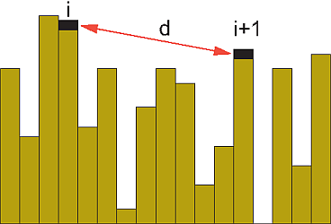|\n",
"\n",
"**Figure 16.6** *A:* A view that might be seen in the undergrowth of a\n",
"forest or after a correlated ballistic deposition. *B:* The probability of\n",
"particle $\\textit{i} + \\text{1}$ sticking in one column depends upon the distance\n",
"*d* from the previously deposited particle *i*.\n",
"\n",
"As in our study of uncorrelated deposition, a uniform random number in\n",
"the interval $[0,L]$ determines the column in which the particle will be\n",
"deposited. We use the same rules about the heights as before, but now a\n",
"second random number is used in conjunction with (16.27) to decide if\n",
"the particle will stick. For instance, if the computed probability is\n",
"$0.6$ and if $r <0.6$, the particle will be accepted (sticks), if $r\n",
">0.6$, the particle will be rejected."
]
},
{
"cell_type": "markdown",
"metadata": {},
"source": [
"## 16.7 Globular Cluster (Problem 6) \n",
"\n",
"Consider a bunch of grapes on an overhead vine. Your **problem** is to\n",
"determine how its tantalizing shape arises. In a flash of divine\n",
"insight, you realize that these shapes, as well as others such as those\n",
"of dendrites, colloids, and thin-film structure, appear to arise from an\n",
"aggregation process that is limited by diffusion.\n",
"\n",
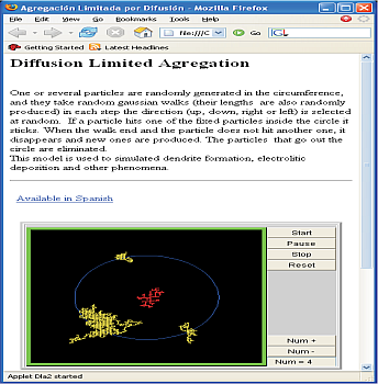
"### 16.7.1 Diffusion-Limited Aggregation Algorithm\n",
"\n",
"A model of diffusion-limited aggregation (DLA) has successfully\n",
"explained the relation between a cluster’s perimeter and mass \\[[Witten &\n",
"Sander(83)](BiblioLinked.html#witt)\\]. We start with a 2-D lattice containing a seed particle in\n",
"the middle, draw a circle around the particle, and place another\n",
"particle on the circumference of the circle at some random angle. We\n",
"then release the second particle and have it execute a random walk, much\n",
"like the one we studied in [Chapter 4, *Monte Carlo: Randomness, Walks &\n",
"Decays*](CP04.ipynb), but restricted to vertical or horizontal jumps\n",
"between lattice sites. This is a simulation of a type of *Brownian\n",
"motion* related to diffusion. To make the model more realistic, we let\n",
"the length of each step vary according to a random Gaussian\n",
"distribution. If at some point during its random walk, the particle\n",
"encounters another particle within one lattice spacing, they stick\n",
"together and the walk terminates. If the particle passes outside the\n",
"circle from which it was released, it is lost forever. The process is\n",
"repeated as often as desired and results in clusters (Figure 16.7 and\n",
"applet `dla`).\n",
"\n",
"|A |B |\n",
"|:- - -:|:- - -:| \n",
"|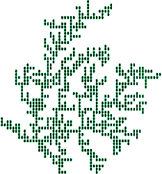||\n",
"\n",
"**Figure 16.7** *A:* A globular cluster of particles of the type that might occur in a colloid. *B:* The applet **Dla2en.html** lets a user watch these clusters grow. Here the cluster is at the center of the circle, and random walkers are started at random points around the circle.\n",
"\n",
"[**Listing 16.2 Column.py**](http://www.science.oregonstate.edu/~rubin/Books/CPbook/Codes/PythonCodes/Fractals/Column.py) simulates correlated ballistic deposition of minerals onto substrates on which dendrites form.\n",
"\n",
"1. Write a subroutine that generates random numbers with a Gaussian\n",
" distribution.\\[*Note:* We indicated how to do this in §5.22.1.\\]\n",
"\n",
"2. Define a 2-D lattice of points represented by the array\n",
" `grid[400,400]` with all elements initially zero.\n",
"\n",
"3. Place the seed at the center of the lattice; that is, set\n",
" `grid[199,199]=1`.\n",
"\n",
"4. Imagine a circle of radius $180$ lattice spacings centered at\n",
" `grid[199,199]`. This is the circle from which we release particles.\n",
"\n",
"\n",
"5. Determine the angular position of the new particle on the circle’s\n",
" circumference by generating a uniform random angle between $0$ and\n",
" $2\\pi$.\n",
"\n",
"6. Compute the $x$ and $y$ positions of the new particle on the circle.\n",
"\n",
"7. Determine whether the particle moves horizontally or vertically by\n",
" generating a uniform random number $0 0.5, & \\mbox{motion is horizontal.}\n",
" \\end{cases}$$\n",
"\n",
"8. Generate a Gaussian-weighted random number in the interval\n",
" $[-\\infty,\\infty]$. This is the size of the step, with the sign\n",
" indicating direction.\n",
"\n",
"9. We now know the total distance and direction the particle will move.\n",
" It jumps one lattice spacing at a time until this total distance\n",
" is covered.\n",
"\n",
"10. Before a jump, check whether a nearest-neighbor site is occupied:\n",
"\n",
" - If occupied, the particle stays at its present position and the\n",
" walk is over.\n",
"\n",
" - If unoccupied, the particle jumps one lattice spacing.\n",
"\n",
" - Continue the checking and jumping until the total distance is\n",
" covered, until the particle sticks, or until it leaves\n",
" the circle.\n",
"\n",
"11. Once one random walk is over, another particle can be released and\n",
" the process repeated. This is how the cluster grows.\n",
"\n",
"Because many particles are lost, you may need to generate hundreds of\n",
"thousands of particles to form a cluster of several hundred particles."
]
},
{
"cell_type": "markdown",
"metadata": {},
"source": [
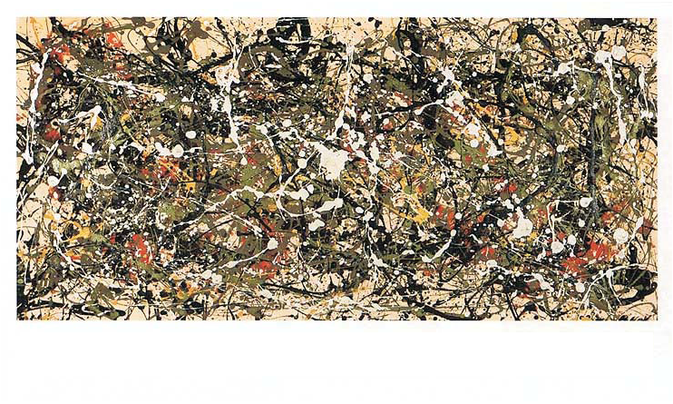
"### 16.7.2 Fractal Analysis of DLA or a Pollock\n",
"\n",
" \n",
"\n",
"**Figure 16.8** Number 8 by the American\n",
"painter Jackson Pollock. (Used with permission, Neuberger Museum, State\n",
"University of New York.) Some researchers claim that Pollock’s paintings\n",
"exhibit a characteristic fractal structure, while some other researchers\n",
"question this \\[[Kennedy(06)](BiblioLinked.html#pollock)\\]. See if you can determine the fractal\n",
"dimensions within this painting.\n",
"\n",
"A cluster generated with the DLA technique is shown in Figure 16.7. We\n",
"wish to analyze it to see if the structure is a fractal and, if so, to\n",
"determine its dimension. (As an alternative, you may analyze the fractal\n",
"nature of the Pollock painting in Figure 13.8, a technique used to\n",
"determine the authenticity of this sort of art.) As a control,\n",
"*simultaneously* analyze a geometric figure, such as a square or circle,\n",
"whose dimension is known. The analysis is a variation of the one used to\n",
"determine the length of the coastline of Britain.\n",
"\n",
"1. If you have not already done so, use the box counting method to\n",
" determine the fractal dimension of a simple square.\n",
"\n",
"2. Draw a square of length $L$, small relative to the size of the\n",
" cluster, around the seed particle. (Small might be seven lattice\n",
" spacings to a side.)\n",
"\n",
"3. Count the number of particles within the square.\n",
"\n",
"4. Compute the density $\\rho$ by dividing the number of particles by\n",
" the number of sites available in the box (49 in our example).\n",
"\n",
"5. Repeat the procedure using larger and larger squares.\n",
"\n",
"6. Stop when the cluster is covered.\n",
"\n",
"7. The (box counting) fractal dimension $d_f$ is estimated from a\n",
" log-log plot of the density $\\rho$ *versus* $L$. If the cluster is a\n",
" fractal, then (16.2) tells us that $\\rho \\propto L^{d_f-2}$, and the\n",
" graph should be a straight line of slope $d_f-2$.\n",
"\n",
"The graph we generated had a slope of $-0.36$, which corresponds to a\n",
"fractal dimension of $1.66$. Because random numbers are involved, the\n",
"graph you generate will be different, but the fractal dimension should\n",
"be similar. (Actually, the structure is multifractal, and so the\n",
"dimension also varies with position.)"
]
},
{
"cell_type": "markdown",
"metadata": {},
"source": [
"## 16.8 Fractals in Bifurcation Plot (Problem 7) \n",
"\n",
"Recollect the project involving the logistics map where we plotted the\n",
"values of the stable population numbers *versus* the growth parameter\n",
"$\\mu$. Take one of the bifurcation graphs you produced and determine the\n",
"fractal dimension of different parts of the graph by using the same\n",
"technique that was applied to the coastline of Britain.\n",
"\n",
"| | |\n",
"|:- - -:|:- - -:| \n",
"|||\n",
"\n",
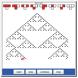
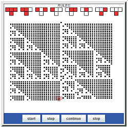
"**Figure 16.9** The rules for two versions of the Game of Life. The rules, given\n",
"graphically on the top row, create the gaskets below. (Output obtained from the\n",
"applet JCellAut in the auxiliary files.)\n",
"\n",
"## 16.9 Fractals from Cellular Automata \n",
"\n",
"*We have already indicated in places how statistical models may lead to\n",
"fractals. There is a class of statistical models known as cellular\n",
"automata that produce complex behaviors from very simple systems.\n",
"Here we study some.*\n",
"\n",
"Cellular automata were developed by von Neumann and Ulam in the early\n",
"1940s (von Neumann was also working on the theory behind modern\n",
"computers then). Though very simple, cellular automata have found\n",
"applications in many branches of science \\[[Peitgen et al.(94)](BiblioLinked.html#peit),\n",
"[Sipper(96)](BiblioLinked.html#cells)\\]. Their classic definition is \\[[Barnsley & Hurd(92)](BiblioLinked.html#barns)\\]:\n",
"\n",
"> *A cellular automaton is a discrete dynamical system in which space,\n",
"> time, and the states of the system are discrete. Each point in a\n",
"> regular spatial lattice, called a cell, can have any one of a finite\n",
"> number of states, and the states of the cells in the lattice are\n",
"> updated according to a local rule. That is, the state of a cell at a\n",
"> given time depends only on its won state one time step previously, and\n",
"> the states of its nearby neighbors at the previous time step. All\n",
"> cells on the lattice are updated synchronously, and so the state of\n",
"> the entice lattice advances in discrete time steps.*\n",
"\n",
"| | |\n",
"|---|---|\n",
"||[Cellular Automata Applet](http://science.oregonstate.edu/~rubin/Books/CPbook/eBook/Applets/index.html)|\n",
"\n",
"A cellular automaton in two dimensions consists of a number of square\n",
"cells that grow upon each other. A famous one is *Conway’s Game of\n",
"Life*, which we implement in Listing 16.3. In this, cells with value 1\n",
"are alive, while cells with value 0 are dead. Cells grow according to\n",
"the following rules:\n",
"\n",
"1. If a cell is alive and if two or three of its eight neighbors are\n",
" alive, then the cell remains alive.\n",
"\n",
"2. If a cell is alive and if more than three of its eight neighbors are\n",
" alive, then the cell dies because of overcrowding.\n",
"\n",
"3. If a cell is alive and only one of its eight neighbors is alive,\n",
" then the cell dies of loneliness.\n",
"\n",
"4. If a cell is dead and more than three of its neighbors are alive,\n",
" then the cell revives.\n",
"\n",
"A variation on the Game of Life is to include a “rule one out of eight”\n",
"that a cell will be alive if exactly one of its neighbors is alive,\n",
"otherwise the cell will remain unchanged.\n",
"\n",
"[**Listing 16.3 Gameoflife.py**](http://www.science.oregonstate.edu/~rubin/Books/CPbook/Codes/PythonCodes/Fractals/Gameoflife.py) is an extension of Conway’s Game of Life in\n",
"which cells always revive if one out of eight neighbors is alive.\n",
"\n",
"Early studies of the statistical mechanics of cellular automata were\n",
"made by \\[[Wolfram(83)](BiblioLinked.html#vold)\\], who indicated how one can be used to generate a\n",
"Sierpiński gasket. Because we have already seen that a Sierpiński gasket\n",
"exhibits fractal geometry (§16.2), this represents a microscopic model\n",
"of how fractals may occur in nature. This model uses eight rules, given\n",
"graphically at the top of Figure 16.9, to generate new cells from old.\n",
"We see all possible configurations for three cells in the top row, and\n",
"the begetted next generation in the row below. At the bottom of\n",
"Figure 16.9 is a Sierpiński gasket of the type created by the applet\n",
"`JCellAut`. This plays the game and lets you watch and control the\n",
"growth of the gasket."
]
},
{
"cell_type": "markdown",
"metadata": {},
"source": [
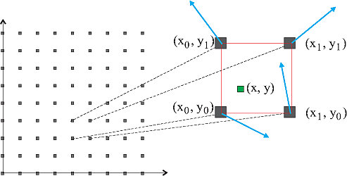
"## 16.10 Perlin Noise Adds Realism $\\odot$ \n",
"\n",
"*We have already seen in this chapter how statistical fractals are able\n",
"to generate objects with a striking resemblance to those in nature. This\n",
"appearance of realism may be further enhanced by including a type of\n",
"coherent randomness known as *Perlin noise*. The technique we are about\n",
"to discuss was developed by Ken Perlin of New York University, who won\n",
"an Academy Award (an Oscar) in 1997 for it and has continued to improve\n",
"it \\[[Perlin(85)](BiblioLinked.html#perlin)\\]. This type of coherent noise has found use in\n",
"important physics simulations of stochastic media \\[[Tickner(04)](BiblioLinked.html#tickner)\\], as\n",
"well as in video games and motion pictures like *Tron*.*\n",
"\n",
"|A| |B| \n",
"|:- - -:|:- - -:| :- - -:| \n",
"| | ||\n",
"\n",
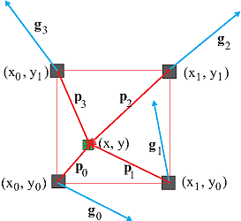
"**Figure 16.10** The coordinates used in adding Perlin noise. *Top:* The\n",
"rectangular grid used to locate a square in space and a corresponding point\n",
"within the square. As shown with the arrows, unit vectors\n",
"$\\mathbf{g}_{\\textit{i}}$ with random orientation are assigned at each grid\n",
"point. *Bottom:* A point within each square is located by drawing the four\n",
"$\\mathbf{p}_{\\textit{i}}$. The $\\mathbf{g}_{\\textit{i}}$ vectors are the same as\n",
"on the left.\n",
"\n",
"The inclusion of Perlin noise in a simulation adds both randomness and a\n",
"type of coherence among points in space that tends to make dense regions\n",
"denser and sparse regions sparser. This is similar to our correlated\n",
"ballistic deposition simulations (§16.6.1) and related to chaos in its\n",
"long-range randomness and short-range correlations. We start with some\n",
"known function of $x$ and $y$ and add noise to it. For this purpose\n",
"Perlin used the mapping or *ease* function (Figure 16.11 B)\n",
"\n",
"$$\\tag*{16.29} f(p)= 3p^2-2p^3.$$\n",
"\n",
"As a consequence of its S shape, this mapping makes regions close to 0 even\n",
"closer to 0, while making regions close to 1 even closer (in other words, it\n",
"increases the tendency to clump, which shows up as higher contrast). We then\n",
"break space up into a uniform rectangular grid of points (Figure 16.10 top), and\n",
"consider a point $(x,y)$ within a square with vertices $(x_0,y_0)$, $(x_1,y_0)$,\n",
"$(x_0,y_1)$, and $(x_1,y_1)$. We next assign unit gradients vectors\n",
"$\\mathbf{g}_0$ to $\\mathbf{g}_3$ with random orientation at each grid point.\n",
"A point within each square is located by drawing the four $\\mathbf{p}_i$\n",
"vectors (Figure 16.10 bottom):\n",
"\n",
"$$\\begin{align}\n",
"\\tag*{16.30}\n",
"\\mathbf{p}_0 = (x-x_0) \\mathbf{i} + (y-y_0)\\mathbf{j}, \\quad &&\n",
"\\mathbf{p}_1 = (x-x_1) \\mathbf{i} + (y-y_0)\\mathbf{j}, \\\\\n",
"\\mathbf{p}_2 = (x-x_1) \\mathbf{i} + (y-y_1)\\mathbf{j}, \\quad &&\n",
"\\mathbf{p}_3 = (x-x_0) \\mathbf{i} + (y-y_1)\\mathbf{j}.\\tag*{16.31}\\end{align}$$\n",
"\n",
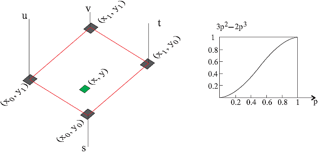
"Next the scalar products of the $\\mathbf{p'}$s and the $\\mathbf{g'}$s\n",
"are formed:\n",
"\n",
"$$\\tag*{16.32} s=\\mathbf{p}_0 \\cdot \\mathbf{g}_0, \\quad\n",
"t=\\mathbf{p}_1\\cdot\n",
"\\mathbf{g}_1, \\quad v=\\mathbf{p}_2\\cdot \\mathbf{g}_2, \\quad\n",
"u=\\mathbf{p}_3\\cdot \\mathbf{g}_3.$$\n",
"\n",
"As shown on the left in Figure 16.11, the numbers $s$, $t$, $u$, and $v$\n",
"are assigned to the four vertices of the square and represented there by\n",
"lines perpendicular to the square with lengths proportional to the\n",
"values of $s$, $t$, $u$, and $v$ (which can be positive or negative).\n",
"\n",
"\n",
"\n",
"**Figure 16.11** The mapping used in adding Perlin noise. *Top:* The numbers $\\textit{s}$, $\\textit{t}$, $\\textit{u}$, and $\\textit{v}$ are represented by perpendiculars to the four vertices, with lengths proportional to their values. *Bottom:* The function $\\text{3}\\textit{p}^{\\text{2}} - \\text{2}\\textit{p}^{\\text{3}}$ is used as a map of the noise at a point like $\\text{(}\\textit{x,} \\textit{y}\\text{)}$ to others close by.\n",
"\n",
"\n",
"\n",
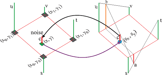
"**Figure 16.12** Perlin noise mapping. *Left*: The point (*x, y*) is mapped to point ($\\textit{s}_{\\textit{x}}, \\textit{x}_{\\textit{y}}$). *Right*: Using (16.33). Then three linear interpolations are performed to find *c*, the noise at (*x, y*).\n",
" \n",
"The actual mapping proceeds via a number of steps (Figure 16.12):\n",
"\n",
"1. Transform the point $(x,y)$ to $(s_x,s_y)$, $$\\tag*{16.33}\n",
" s_x = 3x^2 -2x^3, \\quad s_y = 3y^2 -2y^3.$$\n",
"\n",
"2. Assign the lengths $s$, $t$, $u$, and $v$ to the vertices in the\n",
" mapped square.\n",
"\n",
"3. Obtain the height $a$ (Figure 16.12) via linear interpolation\n",
" between $s$ and $t$.\n",
"\n",
"4. Obtain the height $b$ via linear interpolation between $u$ and $v$.\n",
"\n",
"5. Obtain $s_y$ as a linear interpolation between $a$ and $b$.\n",
"\n",
"6. The vector $c$ so obtained is now the two components of the noise at\n",
" $(x,y)$.\n",
"\n",
"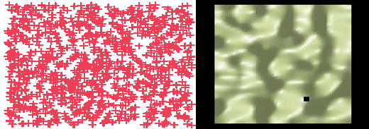\n",
"\n",
"**Figure 16.13** After the addition of Perlin noise, the random scatterplot on\n",
"the left becomes the clusters on the right.\n",
"\n",
"### 16.10.1 Ray Tracing Algorithms\n",
"\n",
"Ray tracing is a technique that renders an image of a scene by\n",
"simulating the way rays of light travel \\[Pov-Ray(13)\\]. ray-tracing\n",
"programs start at the viewer, trace rays backward onto the scene, and\n",
"then back again onto the light sources. You can vary the location of the\n",
"viewer and light sources and the properties of the objects being viewed,\n",
"as well as atmospheric conditions such as fog, haze, and fire.\n",
"\n",
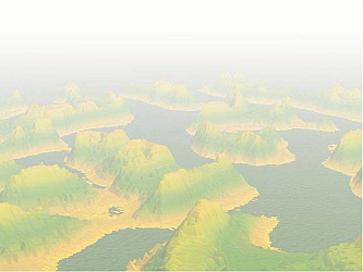
"As an example of what can be carried out, on the left in Figure 16.14 we\n",
"show the output from the ray-tracing program `Islands.poc` in\n",
"Listing 16.4, using as input the coherent random noise on the right in\n",
"Figure 16.13. The program options we used are given in the program and\n",
"are seen to include commands to color the islands, to include waves, and\n",
"to give textures to the sky and the sea. Pov-Ray also allows the\n",
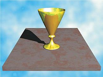
"possibility of using Perlin noise to give textures to the objects to be\n",
"created. For example, the stone cup on the right in Figure 16.14 has a\n",
"marblelike texture produced by Perlin noise.\n",
"\n",
"| | | \n",
"|:- - -:|:- - -:|\n",
"|| |\n",
"\n",
"**Figure 16.14** *A:* The output from the Pov-Ray ray-tracing program that\n",
"took as input the 2-D coherent random noise plot in Figure 16.13 and added\n",
"height and fog. *B:* An image of a surface of revolution produced by\n",
"Pov-Ray in which the marblelike texture is created by Perlin noise.\n",
"\n",
"[**Listing 16.4 Islands.pov**](http://www.science.oregonstate.edu/~rubin/Books/CPbook/Codes/Animations/Fractals/Islands.pov) in the Codes/Animations/Fractals/ directory gives\n",
"the Pov-Ray ray-tracing commands needed to convert the\n",
"coherent noise random plot of Figure 16.13 into the mountain-like image in\n",
"Figure 16.14 left."
]
},
{
"cell_type": "markdown",
"metadata": {
"collapsed": true
},
"source": [
"## 16.11 Exercises \n",
"\n",
"1. Figure 16.9 gives the rules (at top) and the results (below) for two\n",
" versions of the Game of Life. These results were produced by the\n",
" applet `JCellAut`. Write a Python program that runs the same games.\n",
" Check that you obtain the same results for the same\n",
" initial conditions.\n",
"\n",
"2. Recall how box counting is used to determine the fractal dimension\n",
" of an object. Imagine that the result of some experiment or\n",
" simulation is an interesting geometric figure.\n",
"\n",
" - What might be the physical/theoretical importance of determining\n",
" that this object is a fractal?\n",
"\n",
" - What might be the importance of determining its fractal\n",
" dimension?\n",
"\n",
" - Why is it important to use *more* than two sizes of\n",
" boxes?"
]
},
{
"cell_type": "code",
"execution_count": null,
"metadata": {
"collapsed": true
},
"outputs": [],
"source": []
}
],
"metadata": {
"kernelspec": {
"display_name": "Python 2",
"language": "python",
"name": "python2"
},
"language_info": {
"codemirror_mode": {
"name": "ipython",
"version": 2
},
"file_extension": ".py",
"mimetype": "text/x-python",
"name": "python",
"nbconvert_exporter": "python",
"pygments_lexer": "ipython2",
"version": "2.7.11"
}
},
"nbformat": 4,
"nbformat_minor": 0
}