{
"cells": [
{
"cell_type": "markdown",
"metadata": {},
"source": [
"# *Chapter 20*
Heat Flow via Time Stepping \n",
"\n",
"| | | |\n",
"|:---:|:---:|:---:|\n",
"| |[From **COMPUTATIONAL PHYSICS**, 3rd Ed, 2015](http://physics.oregonstate.edu/~rubin/Books/CPbook/index.html)
RH Landau, MJ Paez, and CC Bordeianu (deceased)
Copyrights:
[Wiley-VCH, Berlin;](http://www.wiley-vch.de/publish/en/books/ISBN3-527-41315-4/) and [Wiley & Sons, New York](http://www.wiley.com/WileyCDA/WileyTitle/productCd-3527413154.html)
R Landau, Oregon State Unv,
MJ Paez, Univ Antioquia,
C Bordeianu, Univ Bucharest, 2015.
Support by National Science Foundation.|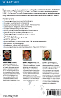|\n",
"\n",
">*As the present now will later be past
\n",
">The order is rapidly fadin’
\n",
">And the first one now will later be last
\n",
">For the times they are a-changin’. * - Bob Dylan\n",
"\n",
"**20 Heat Flow via Time Stepping**
\n",
"[20.1 Heat Flow via Time-Stepping (Leapfrog)](#20.1)
\n",
"[20.2 The Parabolic Heat Equation (Theory)](#20.2)
\n",
" [20.2.1 Solution: Analytic Expansion](#20.2.1)
\n",
" [20.2.2 Solution: Time-Stepping](#20.2.2)
\n",
" [20.2.3 Von Neumann Stability Assessment](#20.2.3)
\n",
" [20.2.4 Heat Equation Implementation](#20.2.4)
\n",
"[20.3 Assessment and Visualization](#20.3)
\n",
"[20.4 Improved Heat Flow: Crank-Nicolson Method](#20.4)
\n",
" [20.4.1 Solution of Tridiagonal Matrix Equations](#20.4.1)
\n",
" [20.4.2 Implementation, Assessment](#20.4.2)
\n",
" \n",
" *In this chapter examine the heat equation and develop the leapfrog\n",
"method for solving it on a space-time lattice. We also develop an\n",
"improved Crank-Nicolson method that determines the solution over all of\n",
"space in a single step. Time stepping is simple, yet important, and we\n",
"will see it again when we attack various wave equations.*\n",
"\n",
"** This Chapter’s Lecture, Slide Web Links, Applets & Animations**\n",
"\n",
"| | |\n",
"|---|---|\n",
"|[All Lectures](http://physics.oregonstate.edu/~rubin/Books/CPbook/eBook/Lectures/index.html)|[](http://physics.oregonstate.edu/~rubin/Books/CPbook/eBook/Lectures/index.html)|\n",
"\n",
"|*Lecture (Flash)*| *Slides* | *Sections*|*Lecture (Flash)*| *Slides* | *Sections*| \n",
"|- - -|:- - -:|:- - -:|- - -|:- - -:|:- - -:|\n",
"|[Intro to PDE’s](http://science.oregonstate.edu/~rubin/Books/CPbook/eBook/VideoLecs/PDE_Intro/PDE_Intro.html)|[pdf](http://physics.oregonstate.edu/~rubin/Books/CPbook/eBook/Lectures/Slides/Slides_NoAnimate_pdf/PDE's_08Mar.pdf)| 17.1 | [PDE Electrostatics I](http://science.oregonstate.edu/~rubin/Books/CPbook/eBook/VideoLecs/Elec1/Elec1.html)|[pdf](http://physics.oregonstate.edu/~rubin/Books/CPbook/eBook/Lectures/Slides/Slides_NoAnimate_pd/ElectricField_10Mar.pdf)| 17.2 | \n",
"| [Electrostatics II](http://science.oregonstate.edu/~rubin/Books/CPbook/eBook/VideoLecs/Elec2/Elec2.html)|[pdf](http://science.oregonstate.edu/~rubin/Books/CPbook/eBook//Slides/Slides_NoAnimate_pdf/ElectricField_10Mar.pdf)| 17.4 |[Finite Elements Electrostatics](http://science.oregonstate.edu/~rubin/Books/CPbook/eBook/VideoLecs/FEM/FEM.html)|[pdf](http://physics.oregonstate.edu/~rubin/Books/CPbook/eBook/Lectures/Slides/Slides_NoAnimate_pdf/FiniteElements_26May.pdf)| 17.10 | \n",
"| [PDE Heat](http://science.oregonstate.edu/~rubin/Books/CPbook/eBook/VideoLecs/Heat/Heat.html)|[pdf](http://physics.oregonstate.edu/~rubin/Books/CPbook/eBook/Lectures/Slides/Slides_NoAnimate_pdf/Heat_06Ap10.pdf)|17.16|[Heat Crank-N](http://science.oregonstate.edu/~rubin/Books/CPbook/eBook/VideoLecs/Heat_CN/Heat_CN.html)|[pdf](http://physics.oregonstate.edu/~rubin/Books/CPbook/eBook/Lectures/Slides/Slides_NoAnimate_pdf/HeatCrank_96Ap10.pdf)| 17.19|\n",
"|[Heat Equation Applet](http://science.oregonstate.edu/~rubin/Books/CPbook/eBook/Applets/index.html)| | | | |"
]
},
{
"cell_type": "markdown",
"metadata": {},
"source": [
"# 20.1 Heat Flow via Time-Stepping (Leapfrog) \n",
"\n",
"**Problem:** You are given an aluminum bar of length $L=1 \\mbox{m}$ and\n",
"width $w$ aligned along the $x$ axis (Figure 20.1). It is insulated\n",
"along its length but not at its ends. Initially the bar is at a uniform\n",
"temperature of 100 C, and then both ends are placed in contact with ice\n",
"water at 0 C. Heat flows out of the noninsulated ends only. Your\n",
"**problem** is to determine how the temperature will vary as we move\n",
"along the length of the bar at later times.\n",
"\n",
"\n",
"\n",
"**Figure 20.1** A metallic bar insulated along its length with its ends in contact\n",
"with ice. The bar is colored solid red and the insulation is of lighter color.\n",
"\n",
"# 20.2 The Parabolic Heat Equation (Theory) \n",
"\n",
"A basic fact of nature is that heat flows from hot to cold, that is,\n",
"from regions of high temperature to regions of low temperature. We give\n",
"these words mathematical expression by stating that the rate of heat\n",
"flow $\\textbf{H}$ through a material is proportional to the gradient of\n",
"the temperature $T$ across the material:\n",
"\n",
"$$\\tag*{20.1}\n",
"\\textbf{H} =- K \\mathbf{\\nabla} T(\\mathbf{x}, t),$$\n",
"\n",
"where $K$ is the thermal conductivity of the material. The total amount\n",
"of heat $Q(t)$ in the material at any one time is proportional to the\n",
"integral of the temperature over the material’s volume:\n",
"\n",
"$$\\tag*{20.2} Q(t) = \\int d\\textbf{x} C \\rho(\\textbf{x}) T(\\textbf{x}, t),$$\n",
"\n",
"where $C$ is the specific heat of the material and $\\rho$ is its\n",
"density. Because energy is conserved, the rate of decrease in $Q$ with\n",
"time must equal the amount of heat flowing out of the material. After\n",
"this energy balance is struck and the divergence theorem applied, there\n",
"results the *heat equation*:\n",
"\n",
"$$\\tag*{20.3}\n",
"\\frac{\\partial T(\\textbf{x}, t)}{\\partial t} = \\frac{K}{C \\rho}\n",
"\\nabla^2 T(\\textbf{x}, t).$$\n",
"\n",
"The heat equation (20.3) is a parabolic PDE with space and time as\n",
"independent variables. The specification of this problem implies that\n",
"there is no temperature variation in directions perpendicular to the bar\n",
"($y$ and $z$), and so we have only one spatial coordinate in the\n",
"Laplacian:\n",
"\n",
"$$\\tag*{20.4}\n",
"\\frac {\\partial T(x,t)}{\\partial t} = \\frac{K}{C\\rho}\n",
"\\frac{\\partial ^2 T(x,t)}{\\partial x^2}.$$\n",
"\n",
"As given, the initial temperature of the bar and the boundary conditions\n",
"are\n",
"\n",
"$$\\tag*{20.5} T(x,t=0) = 100 \\mbox{C}, \\quad T(x=0,t) = T(x=L,t) = 0\n",
"\\mbox{C}.$$"
]
},
{
"cell_type": "markdown",
"metadata": {},
"source": [
"### 20.2.1 Solution: Analytic Expansion\n",
"\n",
"Analogous to Laplace’s equation, the analytic solution starts with the\n",
"assumption that the solution separates into the product of functions of\n",
"space and time:\n",
"\n",
"$$\\tag*{20.6} T(x,t) = X(x) {\\cal T}(t).$$\n",
"\n",
"When (20.6) is substituted into the heat equation (20.4) and the\n",
"resulting equation is divided by $X(x) {\\cal T}(t)$, two noncoupled\n",
"ODE’s result:\n",
"\n",
"$$\\tag*{20.7}\n",
"\\frac{d^2 X(x)}{dx^2} +k^2X(x) =0, \\qquad \\frac{d {\\cal\n",
"T}(t)}{dt}+k^2 \\frac{C}{C\\rho} {\\cal T}(t) = 0,$$\n",
"\n",
"where $k$ is a constant still to be determined. The boundary condition\n",
"that the temperature equals zero at $x=0$ requires a sine function for\n",
"$X$:\n",
"\n",
"$$\\tag*{20.8} X(x)= A \\sin k x.$$\n",
"\n",
"The boundary condition that the temperature equals zero at $x=L$\n",
"requires the sine function to vanish there:\n",
"\n",
"$$\\tag*{20.9}\n",
"\\sin k L = 0 \\ \\Rightarrow \\ k = k_n = n\\pi/ L , \\quad\n",
"n=1,2,\\ldots.$$\n",
"\n",
"To avoid blow up, the time function must be a decaying exponential with\n",
"$k$ in the exponent:\n",
"\n",
"$$\\tag*{20.10}\n",
" {\\cal T}(t) = e^{-k_{n}^2 t/C\\rho}, \\ \\Rightarrow\n",
"\\ T(x,t) = A_n \\sin k_n x e^{-k_{n}^2\n",
"t/C\\rho},$$\n",
"\n",
"where $n$ can be any integer and $A_n$ is an arbitrary constant. Because\n",
"(20.4) is a linear equation, the most general solution is a linear\n",
"superposition of $X_n(x)T_n(t)$ products for all values of $n$:\n",
"\n",
"$$\\tag*{20.11} T(x,t)=\\sum_{n=1}^\\infty A_n \\sin k_{n} x e^{-k_{n}^2\n",
"t/C\\rho}.$$\n",
"\n",
"The coefficients $A_n$ are determined by the initial condition that at\n",
"time $t=0$ the entire bar has temperature $T=100$ K:\n",
"\n",
"$$T(x,t=0)= 100 \\ \\Rightarrow \\ \\sum_{n=1}^\\infty A_n\\sin k_{n} x\n",
"= 100. \\tag*{20.12}$$\n",
"\n",
"Projecting the sine functions determines $A_n = {4 T_0 }/{n\\pi}$ for $n$\n",
"odd, and so\n",
"\n",
"$$\\tag*{20.13} T(x,t) = \\sum_{n=1,3,\\ldots}^\\infty \\frac{4 T_0}{n\\pi} \\;\\sin k_n x\n",
"e^{-k_n^2 Kt/(C\\rho)}.$$"
]
},
{
"cell_type": "code",
"execution_count": null,
"metadata": {
"collapsed": true
},
"outputs": [],
"source": []
},
{
"cell_type": "markdown",
"metadata": {},
"source": []
},
{
"cell_type": "markdown",
"metadata": {},
"source": [
"### 20.2.2 Solution: Time-Stepping\n",
"\n",
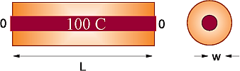
"As we did with Laplace’s equation, the numerical solution is based on\n",
"converting the differential equation to a finite-difference\n",
"(“difference”) equation. We discretize space and time on a lattice\n",
"(Figure 20.2) and solve for solutions on the lattice sites. The sites\n",
"along the top with white centers correspond to the known values of the\n",
"temperature for the initial time, while the sites with white centers\n",
"along the sides correspond to the fixed temperature along the\n",
"boundaries. If we *also* knew the temperature for times along the bottom\n",
"row, then we could use a relaxation algorithm as we did for Laplace’s\n",
"equation. However, with only the top and side rows known, we shall end\n",
"up with an algorithm that steps forward in time one row at a time, as in\n",
"the children’s game *leapfrog*.\n",
"\n",
"\n",
"\n",
"**Figure 20.2** The algorithm for the heat equation in which the temperature\n",
"at the location $\\textit{x}=\\textit{i} \\Delta \\textit{x}$ and time\n",
"$\\textit{t}=(\\textit{j}+\\text{1})\\Delta t$ is computed from the temperature\n",
"values at three points of an earlier time. The nodes with white centers\n",
"correspond to known initial and boundary conditions. (The boundaries are\n",
"placed artificially close for illustrative purposes.)\n",
"\n",
"As is often the case with PDE’s, the algorithm is customized for the\n",
"equation being solved and for the constraints imposed by the particular\n",
"set of initial and boundary conditions. With only one row of times to\n",
"start with, we use a forward-difference approximation for the time\n",
"derivative of the temperature:\n",
"\n",
"$$\\tag*{20.14}\n",
"\\frac{\\partial T(x,t)}{\\partial t} \\simeq \\frac{T(x,t+\\Delta t)-\n",
"T(x,t)}{\\Delta t}.$$\n",
"\n",
"Because we know the spatial variation of the temperature along the\n",
"entire top row and the left and right sides, we are less constrained\n",
"with the space derivative as with the time derivative. Consequently, as\n",
"we did with the Laplace equation, we use the more accurate\n",
"central-difference approximation for the space derivative:\n",
"\n",
"$$\\tag*{20.15}\n",
"\\frac{\\partial^2 T(x,t)}{\\partial x^2} \\simeq \\frac{T(x +\\Delta\n",
"x,t) +T(x-\\Delta x,t)-2 T(x,t)}{(\\Delta x)^2}.$$\n",
"\n",
"Substitution of these approximations into (20.4) yields the heat\n",
"difference equation\n",
"\n",
"$$\\tag*{20.16}\n",
"\\frac{T(x,t+ \\Delta t)-T(x,t)}{\\Delta t} = \\frac{K}{C\\rho}\n",
"\\frac{T(x+\\Delta x,t) +T(x-\\Delta x,t) -2 T(x,t)}{\\Delta\n",
"x^2}.$$\n",
"\n",
"We reorder (20.16) into a form in which $T$ can be stepped forward in\n",
"$t$:\n",
"\n",
"$$\\tag*{20.17}\n",
" T_{i,j+1} = T_{i,j}+ \\eta\n",
"\\left[T_{i+1,j}+T_{i-1,j}-2T_{i,j}\\right], \\quad \\eta = \\frac{K\n",
"\\Delta t}{C\\rho \\Delta x^2},$$\n",
"\n",
"where $x=i \\Delta x$ and $t = j \\Delta t$. This algorithm is *explicit*\n",
"because it provides a solution in terms of known values of the\n",
"temperature. If we tried to solve for the temperature at all lattice\n",
"sites in Figure. 20.2 simultaneously, then we would have an *implicit*\n",
"algorithm that requires us to solve equations involving unknown values\n",
"of the temperature. We see that the temperature at space-time point\n",
"$(i,j+1)$ is computed from the three temperature values at an earlier\n",
"time $j$ and at adjacent space values $i\\pm 1, i$. We start the solution\n",
"at the top row, moving it forward in time for as long as we want and\n",
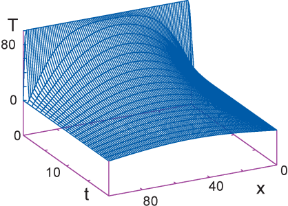
"keeping the temperature along the ends fixed at 0 K (Figure 20.3).\n",
"\n",
" \n",
"\n",
"**Figure 20.3** A numerical calculation of the temperature\n",
"*versus* position and *versus* time, with\n",
"isotherm contours projected onto the horizontal plane.\n",
"\n",
"### 20.2.3 Von Neumann Stability Assessment\n",
"\n",
"When we solve a PDE by converting it to a difference equation, we hope\n",
"that the solution of the latter is a good approximation to the solution\n",
"of the former. If the difference-equation solution diverges, then we\n",
"know we have a bad approximation, but if it converges, then we may feel\n",
"confident that we have a good approximation to the PDE. The *von Neumann\n",
"stability analysis* is based on the assumption that eigenmodes of the\n",
"difference equation can be expressed as\n",
"\n",
"$$\\tag*{20.18} T_{m,j} = \\xi(k)^j e^{ikm\\Delta x},$$\n",
"\n",
"where $x=m \\Delta x$ and $t=j \\Delta t$, and $i=\\sqrt{-1}$ is the imaginary\n",
"number. The constant $k$ in (20.18) is an unknown wave vector\n",
"($2\\pi/\\lambda$), and $\\xi(k)$ is an unknown complex function. View (20.18) as\n",
"a basis function that oscillates in space (the exponential) with an amplitude or\n",
"*amplification factor* $\\xi(k)^j$ that increases by a power of $\\xi$ for each\n",
"time step. If the general solution to the difference equation can be expanded in\n",
"terms of these eigenmodes, then the general solution will be stable if the\n",
"eigenmodes are stable. Clearly, for an eigenmode to be stable, the amplitude\n",
"$\\xi$ cannot grow in time $j$, which means $|xi(k)|<1$ for all values of the\n",
"parameter $k$ \\[[Press et al.(94)](BiblioLinked.html#press), [Ancona(02)](BiblioLinked.html#ancona)\\].\n",
"\n",
"Application of a stability analysis is more straightforward than it\n",
"might appear. We just substitute the expression (20.18) into the\n",
"difference equation (20.17):\n",
"\n",
"$$ \\tag*{20.19}\n",
"\\xi^{j+1} e^{ikm\\Delta x} = \\xi^{j+} e^{ikm\\Delta x} \n",
" +\\eta\n",
"\\left[\\xi^{j} e^{ik(m+1)\\Delta x} + \\xi^{j+} e^{ik(m-1)\\Delta x}\n",
"-2 \\xi^{j+} e^{ikm\\Delta x}\\right] .$$\n",
"\n",
"After canceling some common factors, it is easy to solve for $\\xi$:\n",
"\n",
"$$\\tag*{20.20}\n",
"\\xi(k) = 1 + 2\\eta [\\cos(k\\Delta x)-1] .$$\n",
"\n",
"In order for $|xi(k)|<1$ for all possible $k$ values, we must have\n",
"\n",
"$$\\tag*{20.21}\n",
"\\eta = \\frac{K \\Delta t}{C\\rho \\Delta x^2}\n",
"<\\frac{1}{2}.$$\n",
"\n",
"This equation tells us that if we make the time step $\\Delta t$ smaller,\n",
"we will always improve the stability, as we would expect. But if we\n",
"decrease the space step $\\Delta x$ without a simultaneous quadratic\n",
"*increase* in the time step, we will worsen the stability. The lack of\n",
"space-time symmetry arises from our use of stepping in time, but not in\n",
"space.\n",
"\n",
"In general, you should perform a stability analysis for every PDE you\n",
"have to solve, although it can get complicated \\[Press et al.(94)\\]. Yet\n",
"even if you do not, the lesson here is that you may have to try\n",
"different *combinations* of $\\Delta x$ and $\\Delta t$ variations until a\n",
"stable, reasonable solution is obtained. You may expect, nonetheless,\n",
"that there are choices for $\\Delta x$ and $\\Delta t$ for which the\n",
"numerical solution fails and that simply decreasing an individual\n",
"$\\Delta x$ or $\\Delta t$, in the hope that this will increase precision,\n",
"may not improve the solution.\n",
"\n",
"[**Listing 20.1 EqHeat.py**](http://www.science.oregonstate.edu/~rubin/Books/CPbook/Codes/PythonCodes/EqHeat.py) solves the 1-D space heat equation on a lattice by\n",
"leapfrogging (time-stepping) the initial conditions forward in time. You will need\n",
"to adjust the parameters to obtain a solution like those in the figures."
]
},
{
"cell_type": "code",
"execution_count": null,
"metadata": {
"collapsed": false
},
"outputs": [
{
"name": "stdout",
"output_type": "stream",
"text": [
"Working, wait for figure after count to 30\n",
"1\n",
"2\n",
"3\n",
"4\n",
"5\n",
"6\n",
"7\n",
"8\n",
"9\n",
"10\n",
"11\n",
"12\n",
"13\n",
"14\n",
"15\n",
"16\n",
"17\n",
"18\n",
"19\n",
"20\n",
"21\n",
"22\n",
"23\n",
"24\n",
"25\n",
"26\n",
"27\n",
"28\n",
"29\n",
"30\n"
]
}
],
"source": [
"# EqHeat.py, Notebook Version\n",
"\n",
"#from __future__ import division,print_function\n",
"from IPython.display import IFrame\n",
"from numpy import *\n",
"import numpy as np\n",
"import matplotlib.pylab as p\n",
"from mpl_toolkits.mplot3d import Axes3D ;\n",
"\n",
"Nx = 101; Nt = 9000; Dx = 0.01; Dt = 0.3 \n",
"KAPPA = 210.; SPH = 900.; RHO = 2700. # conductivity, specific heat, density \n",
"T = zeros( (Nx, 2), float); Tpl = zeros( (Nx, 31), float) \n",
" \n",
"print(\"Working, wait for figure after count to 30\")\n",
"\n",
"for ix in range (1, Nx - 1):\n",
" T[ix, 0] = 100.0; # initial temperature\n",
"T[0,0] = 0.0 ; T[0,1] = 0. # first and last points at 0\n",
"T[Nx-1,0] = 0. ; T[Nx-1,1] = 0.0\n",
"cons = KAPPA/(SPH*RHO)*Dt/(Dx*Dx); # constant\n",
"m = 1 # counter for rows, one every 300 time steps\n",
"\n",
"for t in range (1, Nt): # time iteration\n",
" for ix in range (1, Nx - 1): # Finite differences\n",
" T[ix, 1] = T[ix, 0] + cons*(T[ix + 1, 0] + T[ix - 1, 0] - 2.0*T[ix, 0]) \n",
" if t%300 == 0 or t == 1: # for t = 1 and every 300 time steps\n",
" for ix in range (1, Nx - 1, 2): Tpl[ix, m] = T[ix, 1] \n",
" print(m) \n",
" m = m + 1 # increase m every 300 time steps\n",
" for ix in range (1, Nx - 1): T[ix, 0] = T[ix, 1] # 100 positons at t=m\n",
"x = list(range(1, Nx - 1, 2)) # plot every other x point\n",
"y = list(range(1, 30)) # every 10 points in y (time)\n",
"X, Y = p.meshgrid(x, y) # grid for position and time\n",
"\n",
"def functz(Tpl): # Function returns temperature\n",
" z = Tpl[X, Y] \n",
" return z\n",
"\n",
"Z = functz(Tpl) \n",
"fig = p.figure() # create figure\n",
"ax = Axes3D(fig) # plots axis\n",
"ax.plot_wireframe(X, Y, Z, color = 'r') # red wireframe\n",
"ax.set_xlabel('Position') # label axes\n",
"ax.set_ylabel('time')\n",
"ax.set_zlabel('Temperature')\n",
"p.show() # shows figure, close Python shell\n",
"print(\"finished\") "
]
},
{
"cell_type": "markdown",
"metadata": {},
"source": [
"### EqHeatAnimate.py, Notebook Version"
]
},
{
"cell_type": "code",
"execution_count": null,
"metadata": {
"collapsed": false
},
"outputs": [],
"source": [
"# EqHeatAnimate.py, Notebook Version\n",
"\n",
"from __future__ import division,print_function\n",
"from ivisual import *\n",
"#from IPython.display import IFrame\n",
"#import random\n",
"#from numpy import *\n",
"\n",
"scene=canvas(title=\"Heat Equation\")\n",
"scene.width=500\n",
"scene.height=300\n",
"scene.range=100\n",
"\n",
"bar = curve( pos = [( - 100, - 20), (100, - 20)], color = color.magenta ) \n",
"ball1 = sphere( pos = (100, - 20,0), color = color.blue, radius = 4 ) \n",
"ball2 = sphere( pos = ( - 100, - 20,0), color = color.blue, radius = 4 )\n",
"tempe = curve(color = color.red,radius=1)\n",
"Nx = 101 # Grid points in x\n",
"Dx = 0.01414 # x increment\n",
"Dt = 0.6 # t increment\n",
"KAPPA = 210. # Thermal conductivity\n",
"SPH = 900. # Specific heat\n",
"RHO = 2700. # Density\n",
"T = zeros( (Nx, 2), float) # Temp @ first 2 times\n",
"for ix in range (1, Nx - 1): # Initial temperature in the bar\n",
" T[ix, 0] = 100.0 \n",
"T[0,0] = 0.0 # Ends of bar at T = 0\n",
"T[0,1] = 0. \n",
"T[Nx - 1, 0] = 0.\n",
"T[Nx - 1, 1] = 0.0\n",
"cons = KAPPA/(SPH*RHO)*Dt/(Dx*Dx); # Constant combo in algorthim\n",
"'''\n",
"for i in range (0, Nx - 1): \n",
" tempe.x[i] = 2.0*i - 100.0 # Scaled x's\n",
" tempe.y[i] = 0.8*T[i, 0] - 20.0 # Scaled y's (Temp)\n",
"'''\n",
"for a in range(0,2):\n",
" #print(a)\n",
" print(\" cons \",cons)\n",
" rate(50)# Times loop\n",
" for ix in range (1, Nx - 1): # Finite differences\n",
" T[ix,1] = T[ix,0] + cons*(T[ix +1,0]+T[ix-1,0]-2.0*T[ix,0]) \n",
" \n",
" for i in range (0, Nx):\n",
" xx = 2.0*i - 100.0 # Scale 0 -100 -1001*), initialize `T` so that all\n",
" points on the bar except the ends are at 100 K. Set the temperatures\n",
" of the ends to 0 K.\n",
"\n",
"4. Apply (20.14) to obtain the temperature at the next time step.\n",
"\n",
"5. Assign the present-time values of the temperature to the past\n",
" values: `T[i,1] = T[i,2], i = 1, . . . , 101.`\n",
"\n",
"6. Start with 50 time steps. Once you are confident the program is\n",
" running properly, use thousands of steps to see the bar cool\n",
" smoothly with time. For approximately every 500 time steps, print\n",
" the time and temperature along the bar."
]
},
{
"cell_type": "markdown",
"metadata": {},
"source": [
"## 20.3 Assessment and Visualization \n",
"\n",
"1. Check that your program gives a temperature distribution that varies\n",
" smoothly along the bar and agrees with the boundary conditions, as\n",
" in Figure refheat-1.png.\n",
"\n",
"2. Check that your program gives a temperature distribution that varies\n",
" smoothly with time and reaches equilibrium. You may have to vary the\n",
" time and space steps to obtain stable solutions.\n",
"\n",
"3. Compare the analytic and numeric solutions (and the wall times\n",
" needed to compute them). If the solutions differ, suspect the one\n",
" that does not appear smooth and continuous.\n",
"\n",
"4. Make a surface plot of temperature *versus* position *versus* time.\n",
"\n",
"5. Plot the *isotherms* (contours of constant temperature).\n",
"\n",
"6. **Stability test:** Verify the stability condition (20.21) by\n",
" observing how the temperature distribution diverges if\n",
" $\\eta>{\\frac {1}{4}}$.\n",
"\n",
"7. **Material dependence:** Repeat the calculation for iron. Note that\n",
" the stability condition requires you to change the size of the\n",
" time step.\n",
"\n",
"8. **Initial sinusoidal distribution $\\sin(\\pi x/ L)$:** Compare to the\n",
" analytic solution,\n",
"\n",
" $$\\tag*{20.24}\n",
" T(x,t)= \\sin (\\pi x/L) e^{ -\\pi^2 Kt/(L^2 C\\rho)} .$$\n",
"\n",
"9. **Two bars in contact:** Two identical bars 0.25 m long are placed\n",
" in contact along one of their ends with their other ends kept at\n",
" 0 K. One is kept in a heat bath at 100 K, and the other at 50 K.\n",
" Determine how the temperature varies with time and\n",
" location (Figure 20.4).\n",
"\n",
"10. **Radiating bar (Newton’s cooling):** Imagine now that instead of\n",
" being insulated along its length, a bar is in contact with an\n",
" environment at a temperature $T_e$. Newton’s law of\n",
" cooling (radiation) says that the rate of temperature change as a\n",
" result of radiation is\n",
"\n",
" $$\\tag*{20.25}\n",
" \\frac{\\partial T} { \\partial t}=-h(T-T_e),$$\n",
"\n",
" where $h$ is a positive constant. This leads to the modified heat\n",
" equation\n",
"\n",
" $$\\tag*{20.26}\n",
" \\frac{\\partial T(x,t)}{\\partial t}= \\frac{K}{C\\rho}\n",
" \\frac{\\partial^2 T}{\\partial^2 x}-h T(x,t).$$\n",
"\n",
" Modify the algorithm to include Newton’s cooling and compare the\n",
" cooling of a radiating bar with that of the insulated bar.\n",
"\n",
"\n",
"\n",
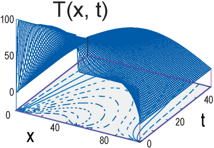
"**Figure 20.4** Temperature *versus* position and time when two bars at\n",
"differing temperatures are placed in contact at $\\textit{t}=\\text{0}$. The\n",
"projected contours show the isotherms.\n",
"\n",
"## 20.4 Improved Heat Flow: Crank-Nicolson Method \n",
"\n",
"The Crank-Nicolson method \\[[Crank & Nicolson(46)](BiblioLinked.html#CN)\\] provides a higher\n",
"degree of precision for the heat equation (20.3) than the simple\n",
"leapfrog method we have just discussed. This method calculates the time\n",
"derivative with a central-difference approximation, in contrast to the\n",
"forward-difference approximation used previously. In order to avoid\n",
"introducing error for the initial time step where only a single time\n",
"value is known, the method uses a *split time step*,\\[*Note:* In §22.2.1\n",
"we develop a different split-time algorithm for the solution of the\n",
"Schrödinger equation. There the real and imaginary parts of the wave\n",
"function are computed at times that differ by $\\Delta t/2$.\\] so that\n",
"time is advanced from time $t$ to $ t+ \\Delta t/2$:\n",
"\n",
"$$\\tag*{20.27} {\\frac{\\partial T}{\\partial t}}\\left(x,t+ \\frac{\\Delta t}{2}\\right)\n",
"\\simeq {\\frac{T(x,t+\\Delta t)-T(x,t)}{\\Delta t}+ O(\\Delta t^2)}.$$\n",
"\n",
"Yes, we know that this looks just like the forward-difference approximation for\n",
"the derivative at time $t+\\Delta t$, for which it would be a bad approximation;\n",
"regardless, it is a better approximation for the derivative at time $t+ \\Delta t/2$,\n",
"although it makes the computation more complicated. Likewise, in (20.14) we\n",
"gave the central-difference approximation for the second space derivative for\n",
"time $t$. For $t= t+ \\Delta t/2$, that becomes \n",
"\n",
"$$\\begin{align}\n",
" & 2 (\\Delta x)^2 {\\frac{\\partial^2 T}{\\partial\n",
"x^2}}\\left(x, t+\\frac{\\Delta t}{2}\\right) \\simeq + \\left[ T(x-\\Delta x, t)-2T(x, t)+T(x+\\Delta x, t)\n",
"\\right] \\\\\n",
" & + [T(x-\\Delta x, t+\\Delta t) - 2T(x, t +\\Delta t)\n",
"+ T(x+\\Delta x, t+\\Delta t)]\n",
" +O(\\Delta x^2).\\tag*{20.28}\\end{align}$$ \n",
" \n",
"In terms of these expressions, the heat difference equation is \n",
"\n",
"$$\\begin{align} T_{i,j+1}-T_{i,j} &=\n",
"\\frac{\\eta} {2}\n",
"\\left[T_{i-1,j+1}-2T_{i,j+1}+T_{i+1,j+1} +\n",
"T_{i-1,j}-2T_{i,j}+T_{i+1,j}\\right],\\\\\n",
" x &=i\\Delta x, \\ t=j\\Delta t, \\\n",
"\\eta=\\frac{K\\Delta t}{C\\rho \\Delta x^2}.\\tag*{20.29}\\end{align}$$ \n",
"\n",
"We\n",
"group together terms involving the same temperature to obtain an\n",
"equation with future times on the LHS and present times on the RHS:\n",
"\n",
"$$\\tag*{20.30}\n",
" -T_{i-1,\n",
"j+1}+\\left(\\frac{2}{\\eta}+2\\right)T_{i, j+1}-T_{i+1, j+1} =\n",
"T_{i-1, j} + \\left(\\frac{2}{\\eta}-2\\right)T_{i, j} + T_{i+1,\n",
"j}.$$\n",
"\n",
"This equation represents an *implicit* scheme for the temperature\n",
"$T_{i,j}$, where the word “implicit” means that we must solve\n",
"simultaneous equations to obtain the full solution for all space. In\n",
"contrast, an *explicit* scheme requires iteration to arrive at the\n",
"solution. It is possible to solve (20.30) simultaneously for all unknown\n",
"temperatures ($1\n",
"\\le i \\le N$) at times $j$ and $j + 1$. We start with the initial\n",
"temperature distribution throughout all of space, the boundary\n",
"conditions at the ends of the bar for all times, and the approximate\n",
"values from the first derivative:\n",
"\n",
"$$\\tag*{20.31}\n",
"\\begin{array}{lll}\n",
"T_{i, 0}, \\mbox{known}, \\quad&T_{0, j}, \\mbox{known}, \\quad &T_{N, j},\n",
"\\mbox{known}, \\\\\n",
"T_{0, j+1} = T_{0, j}=0, &T_{N, j+1}= 0,& T_{N, j}= 0.\n",
"\\end{array}$$\n",
"\n",
"We rearrange (20.30) so that we can use these known values of $T$ to\n",
"step the $j=0$ solution forward in time by expressing (20.30) as a set\n",
"of simultaneous linear equations (in matrix form):\n",
"\n",
"$$\\begin{align} &\\begin{pmatrix} \n",
"\\big(\\frac{2}{\\eta}+2\\big) & -1 & & & & \\\\\n",
" -1 &\\big(\\frac{2}{\\eta}+2\\big) & -1 & & & \\\\\n",
" & -1 & \\big(\\frac{2}{\\eta}+2\\big) & -1 & & \\\\\n",
" & & \\ddots & \\ddots & \\ddots & & \\\\\n",
" & & & -1 &\\big( \\frac{2}{\\eta}+2\\big) &-1 & \\\\\n",
" & & & &-1& \\big(\\frac{2}{\\eta}+2\\big) \\\\\n",
" \\end{pmatrix}\n",
"\\begin{pmatrix}\n",
" T_{1,j+1}\\\\\n",
" T_{2,j+1}\\\\\n",
" T_{3,j+1)}\\\\\n",
" \\vdots \\\\\n",
" T_{n-2,j+1}\\\\\n",
" T_{n-1,j+1}\n",
" \\end{pmatrix} \\\\\n",
" & \\quad =\\begin{pmatrix}\n",
" T_{0,j+1}+T_{0,j}+\\big(\\frac{2}{\\eta}-2\\big)T_{1,j}+T_{2,j}\\\\\n",
" T_{1,j}+\\big(\\frac{2}{\\eta}-2\\big)T_{2,j}+T_{3,j}\\\\\n",
" T_{2,j}+\\big(\\frac{2}{\\eta}-2\\big)T_{3,j}+T_{4,j}\\\\\n",
" \\vdots \\\\\n",
" T_{n-3,j}+\\big(\\frac{2}{\\eta}-2\\big)T_{n-2,j}+T_{n-1,j}\\\\\n",
" T_{n-2,j}+\\big(\\frac{2}{\\eta}-2\\big)T_{n-1,j}+T_{n,j}+T_{n,j+1}\n",
" \\end{pmatrix}. \\tag*{20.32}\\end{align}$$\n",
"\n",
"Observe that the $T$’s on the RHS are all at the present time $j$ for\n",
"various positions, and at future time $j+1$ for the two ends (whose $T$s\n",
"are known for all times via the boundary conditions). We start the\n",
"algorithm with the $T_{i,j=0}$ values of the initial conditions, then\n",
"solve a matrix equation to obtain $T_{i,j=1}$. With that we know all the\n",
"terms on the RHS of the equations ($j=1$ throughout the bar and $j=2$ at\n",
"the ends) and so can repeat the solution of the matrix equations to\n",
"obtain the temperature throughout the bar for $j=2$. So again, we\n",
"time-step forward, only now we solve matrix equations at each step. That\n",
"gives us the spatial solution at all locations directly.\n",
"\n",
"Not only is the Crank-Nicolson method more precise than the low-order\n",
"time-stepping method, but it also is stable for all values of $\\Delta t$ and\n",
"$\\Delta x$. To prove that, we apply the von Neumann stability analysis\n",
"discussed in §20.2.3 to the Crank-Nicolson algorithm by substituting (20.17)\n",
"into (20.30). This determines an amplification factor \n",
"\n",
"$$\\begin{align} \\tag*{20.33}\n",
"\\xi(k) = \\frac{1-2\\eta \\sin^2( {k\\Delta x/2})}{1+2\\eta\n",
"\\sin^2({k\\Delta x/2})}.\\end{align}$$ \n",
"\n",
"Because $\\sin^2()$ is\n",
"positive-definite, this proves that $|xi|\n",
"\\leq 1$ for all $\\Delta t$, $\\Delta x$, and $k$."
]
},
{
"cell_type": "markdown",
"metadata": {},
"source": [
"### 20.4.1 Solution of Tridiagonal Matrix Equations $\\odot$\n",
"\n",
"The Crank-Nicolson equations (20.32) are in the standard\n",
"$[A] \\mathbf{x} = \\mathbf{b}$ form for linear equations, and so we can\n",
"use our previous methods to solve them. Nonetheless, because the\n",
"coefficient matrix $[A]$ is tridiagonal (zero elements except for the\n",
"main diagonal and two diagonals on either side of it),\n",
"\n",
"$$\\begin{pmatrix}\n",
" d_1 & c_1 & 0 & 0 & \\cdots & \\cdots & \\cdots & 0 &\\\\\n",
" a_2 & d_2 & c_2 & 0 & \\cdots & \\cdots & \\cdots & 0 &\\\\\n",
" 0 & a_3 & d_3 & c_3 &\\cdots &\\cdots &\\cdots & 0 &\\\\\n",
" \\cdots & \\cdots & \\cdots & \\cdots & \\cdots & \\cdots & \\cdots & \\cdots\n",
" &\\\\\n",
" 0 & 0 & 0 & 0 &\\cdots & a_{N-1} & d_{N-1} & c_{N-1}\n",
" &\\\\\n",
" 0 & 0 & 0 & 0 & \\cdots & 0 & a_{N} & d_{N} &\n",
" \\end{pmatrix}\n",
"\\begin{pmatrix}\n",
" x_1\\\\\n",
" x_2\\\\\n",
" x_3\\\\\n",
" \\ddots \\\\\n",
" x_{N-1}\\\\\n",
" x_N\n",
" \\end{pmatrix} =\\begin{pmatrix}\n",
" b_1\\\\\n",
" b_2\\\\\n",
" b_3\\\\\n",
" \\ddots \\\\\n",
" b_{N-1}\\\\\n",
" b_N\n",
" \\end{pmatrix},\\tag*{20.34}$$\n",
"\n",
"a more robust and faster solution exists that makes this implicit method\n",
"as fast as an explicit one. Because tridiagonal systems occur\n",
"frequently, we now outline the specialized technique for solving them\n",
"\\[[Press et al.(94)](BiblioLinked.html#press)\\]. If we store the matrix elements $a_{i,j}$ using\n",
"both subscripts, then we will need $N^2$ locations for elements and\n",
"$N^2$ operations to access them. However, for a tridiagonal matrix, we\n",
"need to store only the vectors $\\left\\{d_i\\right\\}_{i=1,N}$,\n",
"$\\left\\{c_i\\right\\}_{i=1,N}$, and $\\left\\{a_i\\right\\}_{i=1,N}$, along,\n",
"above, and below the diagonals. The single subscripts on $a_i$, $d_i$,\n",
"and $c_i$ reduce the processing from $N^2$ to ($3N-2$) elements.\n",
"\n",
"We solve the matrix equation by manipulating the individual equations until the\n",
"coefficient matrix is *upper triangular* with all the elements of the main\n",
"diagonal equal to $1$. We start by dividing the first equation by $d_1$, then\n",
"subtract $a_2$ times the first equation, \n",
"\n",
"$$\\begin{align} &\\begin{pmatrix} 1 &\n",
"\\frac{c_1}{d_1} & 0 & 0 &\\cdots &\\cdots &\\cdots &0 &\\\\\n",
" 0 & d_2-\\frac{a_2c_1}{d_1} & c_2 & 0 & \\cdots &\\cdots & \\cdots & 0 &\\\\\n",
" 0 & a_3 & d_3 & c_3 &\\cdots &\\cdots &\\cdots & 0 &\\\\\n",
" \\cdots & \\cdots & \\cdots & \\cdots & \\cdots & \\cdots & \\cdots & \\cdots&\\\\\n",
" 0 & 0 & 0 & 0 & \\cdots & a_{N-1} & d_{N-1} & c_{N-1} &\\\\\n",
" 0 & 0 & 0 & 0 & \\cdots & 0 & a_{N} & d_{N} &\n",
" \\end{pmatrix}\n",
"\\begin{pmatrix}\n",
" x_1\\\\\n",
" x_2\\\\\n",
" x_3\\\\\n",
" \\ddots \\\\\n",
" \\cdot \\\\\n",
" x_N\n",
" \\end{pmatrix} \n",
" =\\begin{pmatrix}\n",
" \\frac{b_1}{d_1}\\\\\n",
" b_2-\\frac{a_2b_1}{d_1}\\\\\n",
" b_3\\\\\n",
" \\ddots \\\\\n",
" \\cdot\\\\\n",
" b_N\n",
" \\end{pmatrix},&\\tag*{20.35}\\end{align}$$\n",
"\n",
"and then dividing the second equation by the second diagonal element,\n",
"\n",
"$$\\begin{align} \n",
"&\\begin{pmatrix} \n",
"1 & \\frac{c_1}{d_1} & 0 & 0 &\\cdots &\\cdots\n",
"&\\cdots &0 &\\\\\n",
" 0 & 1 &\\frac{ c_2}{d_2-a_2\\frac{c_1}{a_1}} & 0 & \\cdots & & \\cdots & 0 &\\\\\n",
" 0 & a_3 & d_3 & c_3 &\\cdots &\\cdots &\\cdots & 0 &\\\\\n",
" \\cdots & \\cdots & \\cdots & \\cdots & \\cdots & \\cdots & \\cdots & \\cdots&\\\\\n",
" 0 & 0 & 0 & 0 & & a_{N-1} & d_{N-1} & c_{N-1} &\\\\\n",
" 0 & 0 & 0 & 0 & \\cdots & 0 & a_{N} & d_{N} &\n",
" \\end{pmatrix}\n",
"\\begin{pmatrix}\n",
" x_1\\\\\n",
" x_2\\\\\n",
" x_3\\\\\n",
" \\ddots \\\\\n",
" \\cdot \\\\\n",
" x_N\n",
" \\end{pmatrix}\n",
" =\\begin{pmatrix}\n",
" \\frac{b_1}{d_1}\\\\\n",
" \\frac{b_2-a_2\\frac{b_1}{d_1}}{d_2-a_2\\frac{c_1}{d_1}}\\\n",
" b_3\\\\\n",
" \\ddots \\\\\n",
" \\cdot \\\\\n",
" b_N\n",
" \\end{pmatrix}.\\tag*{20.36}\\end{align}$$\n",
"\n",
"Assuming that we can repeat these steps without ever dividing by zero,\n",
"the system of equations will be reduced to upper triangular form,\n",
"\n",
"$$\\tag*{20.37}\n",
"\\begin{pmatrix}\n",
"1 & h_1 & 0 & 0 & \\cdots & 0 &\\\\\n",
" 0 & 1 & h_2 & 0 & \\cdots & 0 &\\\\\n",
" 0 & 0 & 1 & h_3& \\cdots & 0 &\\\\\n",
" 0& \\cdots & \\cdots & \\ddots & \\ddots & \\cdots &\\\\\n",
" 0 & 0 & 0 & 0 & \\cdots & \\cdots &\\\\\n",
" 0 & 0 & 0 & \\cdots & 0 & 1 &\n",
"\\end{pmatrix}\n",
"\\begin{pmatrix}\n",
" x_1\\\\\n",
" x_2\\\\\n",
" x_3\\\\\n",
" \\ddots \\\\\n",
" \\cdot \\\\\n",
" x_N\n",
" \\end{pmatrix} =\\begin{pmatrix}\n",
" p_1\\\\\n",
" p_2\\\\\n",
" p_3\\\\\n",
" \\ddots \\\\\n",
" \\cdot \\\\\n",
" p_N\n",
" \\end{pmatrix},$$\n",
"\n",
"where $h_1 = {c_1}/{d_1}$ and $p_1 = {b_1}/{d_1}$. We then recur for\n",
"the others elements:\n",
"\n",
"$$\\tag*{20.38} h_i=\\frac{c_i}{d_i-a_i h_{i-1}},\\quad\n",
"p_i=\\frac{b_i-a_ip_{i-1}}{d_i-a_i h_{i-1}}.$$\n",
"\n",
"Finally, back substitution leads to the explicit solution for the\n",
"unknowns:\n",
"\n",
"$$\\tag*{20.39} x_i=p_i-h_ix_{i-1}; \\quad i=n-1,n-2,\\ldots ,1 , \\quad x_N=p_N.$$\n",
"\n",
"In Listing 20.2 we give the program `HeatCNTridiag.py` that solves the\n",
"heat equation using the Crank-Nicolson algorithm via a triadiagonal\n",
"reduction.\n",
"\n",
"[**Listing 20.2 HeatCNTridiag.py**](http://www.science.oregonstate.edu/~rubin/Books/CPbook/Codes/PythonCodes/HeatCNTridiag.py) is the complete program for solution of the\n",
"heat equation in one space dimension and time via the Crank-Nicolson method.\n",
"The resulting matrix equations are solved via a technique specialized to\n",
"tridiagonal matrices."
]
},
{
"cell_type": "code",
"execution_count": null,
"metadata": {
"collapsed": false
},
"outputs": [],
"source": [
"# HeatCrankNicolson.py, Notebook Version\n",
"\n",
"from __future__ import division,print_function\n",
"from IPython.display import IFrame\n",
"from numpy import *\n",
"\n",
"import numpy as np\n",
"import matplotlib.pylab as p\n",
"from mpl_toolkits.mplot3d import Axes3D ;\n",
"\n",
"\n",
"Max = 51; n = 50; m = 50\n",
"Ta = zeros( (Max), float ); Tb = zeros( (Max), float ); Tc = zeros((Max), float)\n",
"Td = zeros( (Max), float ); a = zeros( (Max), float ); b = zeros( (Max), float)\n",
"c = zeros( (Max), float ); d = zeros( (Max), float ); x = zeros( (Max), float)\n",
"t = zeros( (Max, Max), float )\n",
"\n",
"def Tridiag(a, d, c, b, Ta, Td, Tc, Tb, x, n): # Define Tridiag method\n",
" Max = 51\n",
" h = zeros( (Max), float )\n",
" p = zeros( (Max), float )\n",
" for i in range(1,n+1):\n",
" a[i] = Ta[i]\n",
" b[i] = Tb[i]\n",
" c[i] = Tc[i]\n",
" d[i] = Td[i]\n",
" h[1] = c[1]/d[1]\n",
" p[1] = b[1]/d[1]\n",
" for i in range(2,n+1):\n",
" h[i] = c[i] / (d[i]-a[i]*h[i-1])\n",
" p[i] = (b[i] - a[i]*p[i-1]) / (d[i]-a[i]*h[i-1])\n",
" x[n] = p[n]\n",
" for i in range( n - 1, 1,-1 ): x[i] = p[i] - h[i]*x[i+1]\n",
"\n",
"width = 1.0; height = 0.1; ct = 1.0 # Rectangle W & H\n",
"for i in range(0, n): t[i,0] = 0.0 # Initialize\n",
"for i in range( 1, m): t[0][i] = 0.0\n",
"h = width / ( n - 1 ) # Compute step sizes and constants\n",
"k = height / ( m - 1 )\n",
"r = ct * ct * k / ( h * h )\n",
"\n",
"for j in range(1,m+1):\n",
" t[1,j] = 0.0\n",
" t[n,j] = 0.0 # BCs\n",
"for i in range( 2, n): \n",
" t[i][1] = sin( pi * h *i) # ICs\n",
"for i in range(1, n+1): \n",
" Td[i] = 2. + 2./r\n",
"Td[1] = 1.\n",
"Td[n] = 1.\n",
"for i in range(1,n ): Ta[i] = -1.0; Tc[i] = -1.0; # Off diagonal\n",
"Ta[n-1] = 0.0; Tc[1] = 0.0; Tb[1] = 0.0; Tb[n] = 0.0\n",
"\n",
"for j in range(2,m+1):\n",
" for i in range(2,n): \n",
" Tb[i] = t[i-1][j-1] + t[i+1][j-1] + (2/r-2) * t[i][j-1]\n",
" Tridiag(a, d, c, b, Ta, Td, Tc, Tb, x, n) # Solve system\n",
" for i in range(1, n+1): \n",
" t[i][j] = x[i]\n",
"print(\"Finished\")\n",
"x = list(range(1, m+1)) # Plot every other x point\n",
"y = list(range(1, n+1)) # every other y point\n",
"X, Y = p.meshgrid(x,y) \n",
"\n",
"def functz(t): # Function returns potential\n",
" z = t[X, Y] \n",
" return z\n",
"Z = functz(t) \n",
"fig = p.figure() # Create figure\n",
"ax = Axes3D(fig) # plots axes\n",
"ax.plot_wireframe(X, Y, Z, color= 'r') # red wireframe\n",
"ax.set_xlabel('t') # label axes\n",
"ax.set_ylabel('x')\n",
"ax.set_zlabel('T')\n",
"p.show() "
]
},
{
"cell_type": "markdown",
"metadata": {
"collapsed": true
},
"source": [
"### 20.4.2 Crank-Nicolson Implementation, Assessment\n",
"\n",
"1. Write a program using the Crank-Nicolson method to solve for the\n",
" heat flow in the metal bar of § 20.1 for at least 100 time steps.\n",
"\n",
"2. Solve the linear system of equations (20.32) using either Matplotlib\n",
" or the special tridiagonal algorithm.\n",
"\n",
"3. Check the stability of your solution by choosing different values\n",
" for the time and space steps.\n",
"\n",
"4. Construct a contoured surface plot of temperature\n",
" *versus* position and versus time.\n",
"\n",
"5. Compare the implicit and explicit algorithms used in this chapter\n",
" for relative precision and speed. You may assume that a stable\n",
" answer that uses very small time steps is accurate."
]
}
],
"metadata": {
"kernelspec": {
"display_name": "Python 2",
"language": "python",
"name": "python2"
},
"language_info": {
"codemirror_mode": {
"name": "ipython",
"version": 2
},
"file_extension": ".py",
"mimetype": "text/x-python",
"name": "python",
"nbconvert_exporter": "python",
"pygments_lexer": "ipython2",
"version": "2.7.11"
}
},
"nbformat": 4,
"nbformat_minor": 0
}