{
"cells": [
{
"cell_type": "markdown",
"metadata": {},
"source": [
"# *Chapter 21*
Wave Equations I: Strings & Membranes \n",
"\n",
"| | | |\n",
"|:---:|:---:|:---:|\n",
"| |[From **COMPUTATIONAL PHYSICS**, 3rd Ed, 2015](http://physics.oregonstate.edu/~rubin/Books/CPbook/index.html)
RH Landau, MJ Paez, and CC Bordeianu (deceased)
Copyrights:
[Wiley-VCH, Berlin;](http://www.wiley-vch.de/publish/en/books/ISBN3-527-41315-4/) and [Wiley & Sons, New York](http://www.wiley.com/WileyCDA/WileyTitle/productCd-3527413154.html)
R Landau, Oregon State Unv,
MJ Paez, Univ Antioquia,
C Bordeianu, Univ Bucharest, 2015.
Support by National Science Foundation.||\n",
"\n",
"**21 Wave Equations I: Strings & Membranes**
\n",
"[21.1 A Vibrating String](#21.1)
\n",
"[21.2 The Hyperbolic Wave Equation (Theory)](#21.2)
\n",
" [21.2.1 Solution via Normal-Mode Expansion](#21.2.1)
\n",
" [21.2.2 Algorithm: Time-Stepping](#21.2.2)
\n",
" [21.2.3 Wave Equation Implementation](#21.2.3)
\n",
" [21.2.4 Assessment, Exploration](#21.2.4)
\n",
"[21.3 Strings with Friction (Extension)](#21.3)
\n",
"[21.4 Strings with Variable Tension & Density](#21.4)
\n",
" [21.4.1 Waves on Catenary](#21.4.1)
\n",
" [21.4.2 Derivation of Catenary Shape](#21.4.2)
\n",
" [21.4.3 Catenary & Frictional Wave Exercises](#21.4.3)
\n",
"[21.5 Vibrating Membrane (2-D Waves)](#21.5)
\n",
"[21.6 Analytical Solution](#21.6)
\n",
"[21.7 Numerical Solution for 2-D Waves](#21.7)
\n",
"\n",
"*In this chapter and the next we explore the numerical solution of\n",
"several PDE’s that yield waves as solutions. If you have skipped the\n",
"discussion of the heat equation in* [Chapter 20, *PDE Review & Heat Flow\n",
"via Time Stepping*](CP20.ipynb),* then this chapter will be the first\n",
"example of how initial conditions are propagated forward in time with a\n",
"time-stepping or leapfrog algorithm. An important aspect of this chapter\n",
"is its demonstration that once you have a working algorithm for solving\n",
"a wave equation, you can include considerably more physics than is\n",
"possible with analytic treatments. First we deal with a number of\n",
"aspects of 1-D waves on a string, and then with 2-D waves on a membrane.\n",
"In the next chapter we look at quantum wave packets and E&M waves. In [Chapter 24](CP23.ipynb) we look at shock and solitary waves.*\n",
"\n",
"** This Chapter’s Lecture, Slide Web Links, Applets & Animations**\n",
"\n",
"| | |\n",
"|---|---|\n",
"|[All Lectures](http://physics.oregonstate.edu/~rubin/Books/CPbook/eBook/Lectures/index.html)|[](http://physics.oregonstate.edu/~rubin/Books/CPbook/eBook/Lectures/index.html)|\n",
"\n",
"| *Lecture (Flash)*| *Slides* | *Sections*|*Lecture (Flash)*| *Slides* | *Sections*| \n",
"|- - -|:- - -:|:- - -:|- - -|:- - -:|:- - -:| \n",
"|[Realistic String Waves](http://physics.oregonstate.edu/~rubin/Books/CPbook/eBook/Lectures/Modules/String/String.html)|[pdf](http://physics.oregonstate.edu/~rubin/Books/CPbook/eBook/Lectures/Slides/Slides_NoAnimate_pdf/WavesStrings_08July.pdf)| 18.1| [Catenary Waves](http://physics.oregonstate.edu/~rubin/Books/CPbook/eBook/Lectures/Modules/Cat_Friction/Cat_Friction.html)|[pdf](http://physics.oregonstate.edu/~rubin/Books/CPbook/eBook/Lectures/Slides/Slides_NoAnimate_pdf/WavesStrings_08July.pdf)|18.3| \n",
"|[Quantum WavePackets](http://science.oregonstate.edu/~rubin/Books/CPbook/eBook/VideoLecs/Quant_Waves/Quant_Waves.html)| [pdf](http://physics.oregonstate.edu/~rubin/Books/CPbook/eBook/Lectures/Slides/Slides_NoAnimate_pdf/WavesQuantum.pdf)|18.5 | [EM Waves (FDTD)](http://physics.oregonstate.edu/~rubin/Books/CPbook/eBook/Lectures/Modules/FDTD/FDTD.html)|[pdf](http://physics.oregonstate.edu/~rubin/Books/CPbook/eBook/Lectures/Slides/Slides_NoAnimate_pdf/FDTD.pdf)|22.5|\n",
"|[Cat with Friction Applet](http://science.oregonstate.edu/~rubin/Books/CPbook/eBook/Movie/CatFrictionAnimate.mov)|-|21.4|[Waves on a String Applet](http://science.oregonstate.edu/~rubin/Books/CPbook/eBook/Applets/index.html)|-| 18.1-18.2 | \n",
"|[String normal mode](http://science.oregonstate.edu/~rubin/Books/CPbook/eBook/Applets/index.html)|-|18.1-18.2 |[Two peaks on a String Applet](http://science.oregonstate.edu/~rubin/Books/CPbook/eBook/Applets/index.html)|-| 18.1-18.2|\n",
"|[Catenary Wave Movie](http://science.oregonstate.edu/~rubin/Books/CPbook/eBook/Movies/CatFrictionAnimate.mov)|-|18.4|[Wavepacket-Wavepacket Scattering Movies](http://science.oregonstate.edu/~rubin/Books/CPbook/eBook/Movies/PacketPackerSymmetrymov.mp4)|-|18.5-18.7 |\n",
"|[Wavepacket Slit Movie](http://science.oregonstate.edu/~rubin/Books/CPbook/eBook/Movies/slitsmall.mpeg)|-| 18.5-18.7| [Square Well Applet](http://science.oregonstate.edu/~rubin/Books/CPbook/eBook/Applets/index.html)|-|18.6 |\n",
"|[Harmonic Oscillator](http://science.oregonstate.edu/~rubin/Books/CPbook/eBook/Applets/index.html)|-|18.7|[Two Slit Interference](http://science.oregonstate.edu/~rubin/Books/CPbook/eBook/Movies/2slits.mp4)|-|18.8|"
]
},
{
"cell_type": "markdown",
"metadata": {},
"source": [
"## 21.1 A Vibrating String \n",
"\n",
"**Problem:** Recall the demonstration from elementary physics in which a\n",
"string tied down at both ends is plucked “gently” at one location and a\n",
"pulse is observed to travel along the string. Likewise, if the string\n",
"has one end free and you shake it just right, a standing-wave pattern is\n",
"set up in which the nodes remain in place and the antinodes move just up\n",
"and down. Your **problem** is to develop an accurate model for wave\n",
"propagation on a string, and to see if you can set up traveling- and\n",
"standing-wave patterns.\\[*Note:* Some similar but independent studies\n",
"can also be found in \\[[Rawitscher et al.(96)](BiblioLinked.html#raw)\\].\\]\n",
"\n",
"## 21.2 The Hyperbolic Wave Equation (Theory) \n",
"\n",
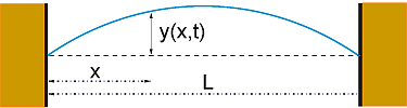
"Consider a string of length $L$ tied down at both ends (Figure 21.1\n",
"left). The string has a constant density $\\rho$ per unit length, a\n",
"constant tension $T$, no frictional forces acting on it, and a tension\n",
"that is so high that we may ignore sagging as a result of gravity. We\n",
"assume that displacement of the string from its rest position $y(x,t)$\n",
"is in the vertical direction only and that it is a function of the\n",
"horizontal location along the string $x$ and the time $t$.\n",
"\n",
"|A|B|\n",
"|:- - -:|:- - -:|\n",
"|||\n",
"\n",
" **Figure 21.1** *A:* A stretched string of length $\\textit{L}$ tied down at both ends\n",
"and under high enough tension so that we can ignore gravity. The vertical\n",
"disturbance of the string from its equilibrium position is\n",
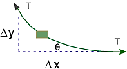
"$\\textit{y}(\\textit{x},\\textit{t})$. *B:* A differential element of the string\n",
"showing how the string’s displacement leads to the restoring force.\n",
"\n",
"To obtain a simple linear equation of motion (nonlinear wave equations are\n",
"discussed in [Chapters 24, *Shock Waves & Solitons*](CP24.ipynb), and [25,\n",
"*Fluid Dynamics*](CP25.ipynb)) we assume that the string’s relative\n",
"displacement $y(x,t)/L$ and slope $\\partial y/\\partial x$ are small. We isolate an\n",
"infinitesimal section $\\Delta x$ of the string (Figure 21.1 right) and see that the\n",
"difference in the vertical components of the tension at either end of the string\n",
"produces the restoring force that accelerates this section of the string in the\n",
"vertical direction. By applying Newton’s laws to this section, we obtain the\n",
"familiar wave equation:\n",
"\n",
"$$\\begin{align} \\tag*{21.1}\n",
"\\sum F_y &= \\rho \\Delta x \\frac{\\partial^2 y}{\\partial t^2}\\\\\n",
"& = T\\sin\\theta(x+\\Delta x) - T\\sin\\theta(x)\\\\ \n",
"& = T \\left. \\frac{\\partial y}{\\partial x}\\right|_{x+\\Delta x} \n",
"- T \\left.\\frac{\\partial y}{\\partial x}\\right|_x \\simeq T \\frac{\\partial^2\n",
"y}{\\partial x^2}, \\tag*{21.3} \\\\\n",
"\\Rightarrow \\quad \\frac{\\partial^2 y(x,t)}{\\partial x^2} & =\n",
"\\frac{1}{c^2} \\frac{\\partial^2 y(x,t)}{\\partial t^2}, \\quad c =\n",
" \\sqrt{\\frac {T}{\\rho}}, \\tag*{21.4}\n",
"\\end{align}$$\n",
" \n",
"where we have assumed\n",
"that $\\theta$ is small enough for\n",
"$\\sin\\theta \\simeq \\tan\\theta =\\partial y/\\partial x$.The existence of\n",
"two independent variables $x$ and $t$ makes this a PDE. The constant $c$\n",
"is the velocity with which a disturbance travels along the wave, and is\n",
"seen to decrease for a denser string and increase for a tighter one.\n",
"Note that this signal velocity $c$ is *not* the same as the velocity of\n",
"a string element $\\partial y/\\partial t$.\n",
"\n",
"The initial condition for our problem is that the string is plucked\n",
"gently and released. We assume that the “pluck” places the string in a\n",
"triangular shape with the center of triangle $\\frac {8}{10}$ of the way\n",
"down the string and with a height of $1$:\n",
"\n",
"$$\\tag*{21.5}\n",
" y(x,t=0)=\\begin{cases}\n",
" 1.25 x/L , &x\\leq 0.8 L ,\\\\\n",
" (5-5x/L), &x> 0.8 L,\n",
" \\end{cases} \\quad \\mbox{(initial condition 1)} .$$\n",
"\n",
"Because (21.4) is second-order in time, a second initial condition\n",
"(beyond initial displacement) is needed to determine the solution. We\n",
"interpret the “gentleness” of the pluck to mean the string is released\n",
"from rest:\n",
"\n",
"$$\\tag*{21.6}\n",
"\\frac{\\partial y} {\\partial t}(x,t=0) =0,\\quad \\mbox{(initial\n",
"condition 2)}.$$\n",
"\n",
"The boundary conditions have both ends of the string tied down for all\n",
"times:\n",
"\n",
"$$\\tag*{21.7} y(0,t) \\equiv 0, \\quad y(L,t) \\equiv 0,\\quad \\mbox{(boundary\n",
"conditions).}$$"
]
},
{
"cell_type": "markdown",
"metadata": {},
"source": [
"### 21.2.1 Solution via Normal-Mode Expansion \n",
"[ Vibrating Spring](http://science.oregonstate.edu/~rubin/Books/CPbook/eBook/Applets/index.html)\n",
"\n",
"The analytic solution to (21.4) is obtained via the familiar\n",
"separation-of-variables technique. We assume that the solution is the\n",
"product of a function of space and a function of time:\n",
"\n",
"$$\\tag*{21.8} y(x,t) = X(x)T(t).$$\n",
"\n",
"We substitute (21.8) into (21.4), divide by $y(x,t)$, and are left with\n",
"an equation that has a solution only if there are solutions to the two\n",
"ODE’s:\n",
"\n",
"$$\\tag*{21.9}\n",
"\\frac{d^2 T(t)}{dt^2} +\\omega^2 T(t) = 0, \\quad \\frac{d^2\n",
"X(x)}{dx^2} +k^2 X(x) = 0,\\quad k { = } \\frac{\\omega}{c}.$$\n",
"\n",
"The angular frequency $\\omega$ and the wave vector $k$ are determined by\n",
"demanding that the solutions satisfy the boundary conditions.\n",
"Specifically, the string being attached at both ends demands\n",
"\n",
"$$\\begin{align}\n",
"\\tag*{21.10}\n",
"& X(x=0,t) = X(x=l,t)=0 \\\\\n",
"\\Rightarrow \\quad X_n(x) =& A_n \\sin {k_n x}, \\quad k_n = \\frac\n",
"{\\pi (n+1) } {L}, \\quad n = 0, 1, \\ldots.\\tag*{21.11}\\end{align}$$\n",
"\n",
"The time solution is\n",
"\n",
"$$\\tag*{21.12} T_n(t) = C_n \\sin \\omega_n t + D_n \\cos \\omega_n t, \\quad\n",
"\\omega_n = n c k_0 = n \\frac{2\\pi c}{L},$$\n",
"\n",
"where the frequency of this $n$th *normal mode* is also fixed. In fact,\n",
"it is the single frequency of oscillation that defines a normal mode.\n",
"The *initial condition* (21.5) of zero velocity,\n",
"$\\partial y/\\partial t (t=0)\n",
"=0$, requires the $C_n$ values in (21.12) to be zero. Putting the pieces\n",
"together, the normal-mode solutions are\n",
"\n",
"$$\\tag*{21.13} y_n(x,t)= \\sin k_nx \\cos \\omega_n t, \\quad n=0, 1,\n",
"\\ldots\\ .$$\n",
"\n",
" \n",
"\n",
"**Figure 21.2** The solutions of the wave\n",
"equation for four earlier space-time points are used to obtain the\n",
"solution at the present time. The boundary and initial conditions are\n",
"indicated by the white-centered dots.\n",
"\n",
"Because the wave equation (21.4) is linear in $y$, the principle of\n",
"linear superposition holds and the most general solution for waves on a\n",
"string with fixed ends can be written as the sum of normal modes:\n",
"\n",
"$$\\tag*{21.14} y(x,t)= \\sum_{n=0}^\\infty B_n \\sin k_nx \\cos \\omega_n t.$$\n",
"\n",
"(Yet we will lose linear superposition once we include nonlinear terms in the\n",
"wave equation.) The Fourier coefficient $B_n$ is determined by the second\n",
"initial condition (21.5), which describes how the wave is plucked:\n",
"\n",
"$$\\tag*{21.15} y(x,t=0)= \\sum_n^\\infty B_n \\sin nk_0x .$$\n",
"\n",
"We multiply both sides by $\\sin mk_0 x$, substitute the value of\n",
"$y(x,0)$ from (21.5), and integrate from 0 to $l$ to obtain\n",
"\n",
"$$\\tag*{21.16} B_m= 6.25 \\;\\frac{\\sin(0.8 m\\pi)} {m^2 \\pi^2}.$$\n",
"\n",
"You will be asked to compare the Fourier series (21.14) to our numerical\n",
"solution. While it is in the nature of the approximation that the\n",
"precision of the numerical solution depends on the choice of step sizes,\n",
"it is also revealing to realize that the precision of the so-called\n",
"analytic solution depends on summing an infinite number of terms, which\n",
"can be carried out only approximately."
]
},
{
"cell_type": "markdown",
"metadata": {},
"source": [
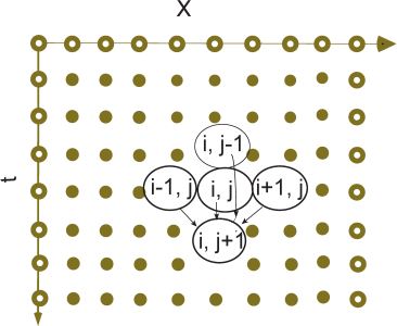
"### 21.2.2 Algorithm: Time-Stepping\n",
"\n",
"As with Laplace’s equation and the heat equation, we look for a solution $y(x,t)$\n",
"only for discrete values of the independent variables $x$ and $t$ on a grid\n",
"(Figure 21.2):\n",
"\n",
"$$\\begin{align} \\tag*{21.17}\n",
"x &=i \\Delta x, \\quad i = 1, \\ldots, N_x, \\quad t = j \\Delta t, \\quad j = 1, \\ldots,\n",
"N_t,\\\\\n",
"y(x,t) &= y(i\\Delta x,\\ i\\Delta t) = y_{i,j}.\\tag*{21.18}\\end{align}$$ \n",
"\n",
"In\n",
"contrast to Laplace’s equation where the grid was in two space dimensions, the\n",
"grid in Figure 21.2 is in both space and time. That being the case, moving across\n",
"a row corresponds to increasing $x$ values along the string for a fixed time,\n",
"while moving down a column corresponds to increasing time steps for a fixed\n",
"position. Although the grid in Figure 21.2 may be square, we cannot use a\n",
"relaxation technique like we did for the solution of Laplace’s equation because\n",
"we do not know the solution on all four sides. The boundary conditions\n",
"determine the solution along the right and left sides, while the initial time\n",
"condition determines the solution along the top.\n",
"\n",
"As with the Laplace equation, we use the central-difference\n",
"approximation to *discretize* the wave equation into a difference\n",
"equation. First we express the second derivatives in terms of finite\n",
"differences:\n",
"\n",
"$$\\tag*{21.19}\n",
"\\frac{\\partial^2 y }{\\partial t^2} \\simeq\n",
"\\frac{y_{i,j+1}+y_{i,j-1}-2 y_{i,j}}{(\\Delta t)^2}, \\quad\n",
"\\frac{\\partial^2 y}{\\partial x^2} \\simeq \\frac{y_{i+1,j}\n",
"+y_{i-1,j}-2 y_{i,j}} {(\\Delta x)^2}.$$\n",
"\n",
"Substituting (21.19) in the wave equation (21.4) yields the difference\n",
"equation\n",
"\n",
"$$\\tag*{21.20}\n",
"\\frac{y_{i,j+1}+y_{i,j-1}-2 y_{i,j}} {c^2 (\\Delta t)^2} =\n",
"\\frac{y_{i+1,j}+y_{i-1,j}-2 y_{i,j}} {(\\Delta x)^2}.$$\n",
"\n",
"Notice that this equation contains three time values: $j+1 = $ the\n",
"future, $j = $ the present, and $j - 1 = $ the past. Consequently, we\n",
"rearrange it into a form that permits us to predict the future solution\n",
"from the present and past solutions:\n",
"\n",
"$$\\tag*{21.21}\n",
" y_{i,j+1} = 2 y_{i,j}-y_{i,j-1}+ \\frac{c^2 }\n",
"{c'^{2}} \\left [ y_{i+1,j}+y_{i-1,j}-2 y_{i,j}\\right], \\quad c'\n",
"{ = } \\frac {\\Delta x}{\\Delta t}.$$\n",
"\n",
"Here $c'$ is a combination of numerical parameters with the dimension of\n",
"velocity whose size relative to $c$ determines the stability of the\n",
"algorithm. The algorithm (21.21) propagates the wave from the two\n",
"earlier times, $j$ and $j-1$, and from three nearby positions, $i-1$,\n",
"$i$, and $i+1$, to a later time $j+1$ and a single space position $i$\n",
"(Figure 21.2).\n",
"\n",
"\n",
"\n",
"**Figure 21.2** The solutions of the wave equation for four earlier space-time\n",
"points are used to obtain the solution at the present time. The boundary and\n",
"initial conditions are indicated by the white-centered dots.\n",
"\n",
"As you have seen in our discussion of the heat equation, a leapfrog\n",
"method is quite different from a relaxation technique. We start with the\n",
"solution along the topmost row and then move down one step at a time. If\n",
"we write the solution for present times to a file, then we need to store\n",
"only three time values on the computer, which saves memory. In fact,\n",
"because the time steps must be quite small to obtain high precision, you\n",
"may want to store the solution only for every fifth or tenth time.\n",
"\n",
"Initializing the recurrence relation is a bit tricky because it requires\n",
"displacements from two earlier times, whereas the initial conditions are\n",
"for only one time. Nonetheless, the rest condition (21.5) when combined\n",
"with the *central-difference* approximation lets us extrapolate to\n",
"negative time:\n",
"\n",
"$$\\tag*{21.22}\n",
"\\frac{\\partial y}{\\partial t}(x,0) \\simeq \\frac{y(x, \\Delta t)- y(x,\n",
"-\\Delta t)}{2\\Delta t}=0, \\ \\Rightarrow \\ y_{i, 0} = y_{i,2}.$$\n",
"\n",
"Here we take the initial time as $j=1$, and so $j=0$ corresponds to\n",
"$t=-\\Delta t$. Substituting this relation into (21.21) yields for the\n",
"initial step\n",
"\n",
"$$\\tag*{21.23} y_{i,2} = y_{i,1}+ \\frac{c^2} {2c'^2} \\left [ y_{i+1,1}+y_{i-1,1}-2\n",
"y_{i,1}\\right] \\quad (\\mbox{for $j=2$ only}).$$\n",
"\n",
"Equation (21.23) uses the solution throughout all space at the initial\n",
"time $t=0$ to propagate (leapfrog) it forward to a time $\\Delta t$.\n",
"Subsequent time steps use (21.21) and are continued for as long as you\n",
"like.\n",
"\n",
"As is also true with the heat equation, the success of the numerical method\n",
"depends on the relative sizes of the time and space steps. If we apply a von\n",
"Neumann stability analysis to this problem by substituting $y_{m,j} = \\xi^j\\exp(i\n",
"k m\\ \\Delta x)$, as we did in §20.2.3, a complicated equation results.\n",
"Nonetheless, \\[[Press et al.(94)](BiblioLinked.html#press)\\] shows that the difference-equation solution will\n",
"be stable for the general class of transport equations if \\[[Courant et al.(28)](BiblioLinked.html#cour)\\]\n",
"\n",
"$$\\begin{align}\n",
"\\tag*{21.24}\n",
"c \\leq c' = {\\Delta x }/ {\\Delta t} \\quad\\mbox{(Courant condition)}.\\end{align}$$\n",
"\n",
"Equation (21.24) means that the solution gets better with smaller *time* steps\n",
"but gets worse for smaller space steps (unless you simultaneously make the time\n",
"step smaller). Having different sensitivities to the time and space steps may\n",
"appear surprising because the wave equation (21.4) is symmetric in $x$ and\n",
"$t$, yet the symmetry is broken by the nonsymmetric initial and boundary\n",
"conditions.\n",
"\n",
"**Exercise:** Figure out a procedure for solving for the wave equation\n",
"for all times in just one step. Estimate how much memory would be\n",
"required.\n",
"\n",
"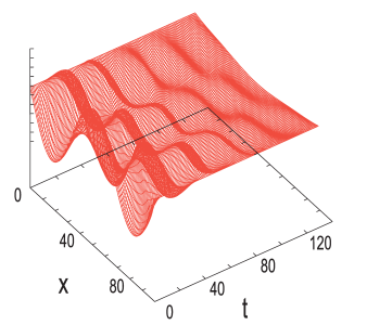\n",
"\n",
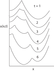
"**Figure 21.3** The vertical displacement as a function of position $x$ and time\n",
"$t$ for a string with friction placed initially in a standing mode (Courtesy of J.\n",
"Wiren.)\n",
"\n",
"**Exercise:** Try to figure out a procedure for solving for the wave\n",
"motion with a relaxation technique. What would you take as your initial\n",
"guess, and how would you know when the procedure has converged?"
]
},
{
"cell_type": "markdown",
"metadata": {},
"source": [
"### EqStringAnimate.py, Notebook Version"
]
},
{
"cell_type": "code",
"execution_count": null,
"metadata": {
"collapsed": false
},
"outputs": [],
"source": [
"#### EqStringAnimate.py, Notebook Version, Vibrating string + MatPlotLib\n",
"\n",
"from numpy import *\n",
"import numpy as np\n",
"import matplotlib.pyplot as plt\n",
"#import scipy.integrate as integrate\n",
"import matplotlib.animation as animation\n",
"\n",
"# Parameters\n",
"rho = 0.01 # string density\n",
"ten = 40. # string tension\n",
"c = sqrt(ten/rho) # Propagation speed\n",
"c1 = c # CFL criterium\n",
"ratio = c*c/(c1*c1)\n",
"# Initialization\n",
"xi = np.zeros( (101, 3), float) # 101 x's & 3 t's \n",
"k=range(0,101)\n",
"def init():\n",
" for i in range(0, 81):\n",
" xi[i, 0] = 0.00125*i # Initial condition: string plucked,shape\n",
" for i in range (81, 101): # first part of string\n",
" xi[i, 0] = 0.1 - 0.005*(i - 80) # second part of string\n",
" \n",
"init() # plot string initial position \n",
"fig=plt.figure() # figure to plot (a changing line)\n",
"# select axis; 111: only one plot, x,y, scales given\n",
"ax = fig.add_subplot(111, autoscale_on=False, xlim=(0, 101), ylim=(-0.15, 0.15))\n",
"ax.grid() # plot a grid\n",
"plt.title(\"Vibrating String\")\n",
"line, = ax.plot(k, xi[k,0], lw=2) # x axis, y values, linewidth=2 \n",
"\n",
"# Later time steps\n",
"for i in range(1, 100): # use algorithm\n",
" xi[i, 1] = xi[i, 0] + 0.5*ratio*(xi[i + 1, 0] + xi[i - 1, 0] - 2*xi[i, 0]) \n",
"\n",
"def animate(num): #num: dummy, algorithm, will plot (x, xi) \n",
" for i in range(1, 100): \n",
" xi[i,2] = 2.*xi[i,1]-xi[i,0]+ratio*(xi[i+1,1]+xi[i-1,1]-2*xi[i,1])\n",
" line.set_data(k,xi[k,2]) # data to plot ,x,y \n",
" for m in range (0,101): # part of algorithm\n",
" xi[m, 0] = xi[m, 1] # recycle array \n",
" xi[m, 1] = xi[m, 2]\n",
" return line,\n",
"# next: animation(figure, function,dummy argument: 1 \n",
"ani = animation.FuncAnimation(fig, animate,1) \n",
"plt.show() \n",
"print(\"finished\")"
]
},
{
"cell_type": "markdown",
"metadata": {},
"source": [
"### 21.2.3 Wave Equation Implementation\n",
"\n",
"The program `EqStringAnimate.py` in Listing 21.1 solves the wave\n",
"equation for a string of length $L=1$ m with its ends fixed and with the\n",
"gently plucked initial conditions. Note that our use of $L=1$ violates\n",
"our assumption that $y/L\\ll 1$ but makes it easy to display the results;\n",
"you should try $L=1000$ to be realistic. The values of density and\n",
"tension are entered as constants, $\\rho=0.01 \\mbox{kg/m}$ and\n",
"$T=40 \\mbox{N}$, with the space grid set at 101 points, corresponding to\n",
"$\\Delta=0.01 $cm.\n",
"\n",
"[**Listing 21.1 EqStringAnimate.py**](http://www.science.oregonstate.edu/~rubin/Books/CPbook/Codes/Animations/VEqStringAnimat.py) solves the wave equation via time\n",
"stepping for a string of length $\\textit{L}=1$ m with its ends fixed and with the\n",
"gently plucked initial conditions. You will need to modify this code to include\n",
"new physics.\n",
"\n",
"### 21.2.4 Assessment, Exploration\n",
"\n",
" 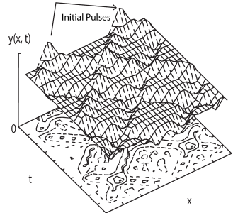\n",
"\n",
"**Figure 21.4** The vertical displacement as a function of position and time of a string initially plucked\n",
" simultaneously at two points, as shown by arrows. Note that each\n",
" initial peak breaks up into waves traveling to the right and to\n",
" the left. The traveling waves invert on reflection from the\n",
" fixed ends. As a consequence of these inversions, the\n",
" $\\textit{t}\\simeq \\text{12}$ wave is an inverted\n",
" $\\textit{t}=\\text{0}$ wave.\n",
" \n",
"1. Solve the wave equation and make a surface plot of displacement\n",
" *versus* time and position.\n",
"\n",
"2. Explore a number of space and time step combinations. In particular,\n",
" try steps that satisfy and that do not satisfy the Courant\n",
" condition (21.24). Does your exploration confirm the stability\n",
" condition?\n",
"\n",
"3. Compare the analytic and numeric solutions, summing at least 200\n",
" terms in the analytic solution.\n",
"\n",
"4. Use the plotted time dependence to estimate the peak’s propagation\n",
" velocity $c$. Compare the deduced $c$ to (21.4).\n",
"\n",
"5. Our solution of the wave equation for a plucked string leads to the\n",
" formation of a wave packet that corresponds to the sum of multiple\n",
" normal modes of the string. On the right in Figure 21.3 we show the\n",
" motion resulting from the string initially placed in a single normal\n",
" mode (standing wave),\n",
"\n",
" $$\\tag*{21.25}\n",
" y(x,t=0) = 0.001 \\sin 2\\pi x, \\quad\\frac{\\partial y}{\\partial\n",
" t}(x,t=0) =0,$$\n",
"\n",
" and with friction (to be discussed soon) included.\n",
"\n",
" Modify your program to incorporate this initial condition and see if\n",
" a normal mode results.\n",
"\n",
"6. Observe the motion of the wave for initial conditions corresponding\n",
" to the sum of two adjacent normal modes. Does beating occur?\n",
"\n",
"7. When a string is plucked near its end, a pulse reflects off the ends\n",
" and bounces back and forth. Change the initial conditions of the\n",
" model program to one corresponding to a string plucked exactly in\n",
" its middle and see if a traveling or a standing wave results.\n",
"\n",
"8. Figure 21.4 shows the wave packets that result as a function of time\n",
" for initial conditions corresponding to the double pluck indicated\n",
" on the left in the figure. Verify that initial conditions of the\n",
" form\n",
"\n",
" $$\\tag*{21.26}\n",
" \\frac{y(x,t=0)}{0.005} =\\begin{cases}\n",
" 0, & 0.0\\leq x \\leq 0.1 , \\\\\n",
" 10x -1, & 0.1 \\leq x \\leq 0.2 ,\\\\\n",
" -10x +3, & 0.2 \\leq x \\leq 0.3 , \\\\\n",
" 0, & 0.3 \\leq x \\leq 0.7 , \\\\\n",
" 10x -7 , & 0.7\\leq x\\leq 0.8 , \\\\\n",
" -10x +9, & 0.8\\leq x \\leq 0.9 ,\\\\\n",
" 0, & 0.9 \\leq x\\leq 1.0\n",
" \\end{cases}$$\n",
"\n",
" lead to this type of a repeating pattern. In particular, observe\n",
" whether the pulses move or just oscillate up and down."
]
},
{
"cell_type": "markdown",
"metadata": {},
"source": [
"## 21.3 Strings with Friction (Extension) \n",
"\n",
"*The string problem we have investigated so far can be handled by either\n",
"a numerical or an analytic technique. We now wish to extend the theory\n",
"to include some more realistic physics. These extensions have only\n",
"numerical solutions.*\n",
"\n",
"Plucked strings do not vibrate forever because there is friction in the\n",
"real world. Consider again the element of a string between $x$ and\n",
"$x + dx$ (Figure 21.1 right) but now imagine that this element is moving\n",
"in a viscous fluid such as air. An approximate model for the frictional\n",
"force has it pointing in a direction opposite the vertical velocity of\n",
"the string and proportional to that velocity, as well as proportional to\n",
"the length of the string element:\n",
"\n",
"$$\\tag*{21.27} F_f \\simeq -2\\kappa\\ \\Delta x\\ \\frac{\\partial y} {\\partial t},$$\n",
"\n",
"where $\\kappa$ is a constant that is proportional to the viscosity of the medium\n",
"in which the string is vibrating. Including this force in the equation of motion\n",
"changes the wave equation to \n",
"\n",
"$$\\begin{align}\n",
"\\tag*{21.28}\n",
"\\frac{\\partial^2y}{\\partial t^2}= c^2 \\frac{\\partial^2\n",
"y}{\\partial x^2} - \\frac{2\\kappa}{\\rho} \\frac{\\partial y}{\\partial t} .\\end{align}$$\n",
"\n",
"In Figure 21.3 we show the resulting motion of a string plucked in the middle\n",
"when friction is included. Observe how the initial pluck breaks up into waves\n",
"traveling to the right and to the left that are reflected and inverted by the fixed\n",
"ends. Because those parts of the wave with the higher velocity experience\n",
"greater friction, the peak tends to be smoothed out the most as time\n",
"progresses.\n",
"\n",
"**Exercise:** Generalize the algorithm used to solve the wave equation\n",
"to now include friction and check if the wave’s behavior seems physical\n",
"(damps in time). Start with $T=40 \\mbox{N}$ and $\\rho=10 \\mbox{kg/m}$,\n",
"and pick a value of $\\kappa$ large enough to cause a noticeable effect\n",
"but not so large as to stop the oscillations. As a check, reverse the\n",
"sign of $\\kappa$ and see if the wave grows in time (which would\n",
"eventually violate our assumption of small oscillations).\n",
"\n",
"## 21.4 Strings with Variable Tension & Density \n",
"\n",
"We have derived the propagation velocity for waves on a string as\n",
"$c=\\sqrt{T/\\rho}$. This says that waves move slower in regions of high\n",
"density and faster in regions of high tension. If the density of the\n",
"string varies, for instance, by having the ends thicker in order to\n",
"support the weight of the middle, then $c$ will no longer be a constant\n",
"and our wave equation will need to be extended. In addition, if the\n",
"density increases, then so will the tension because it takes greater\n",
"tension to accelerate a greater mass. If gravity acts, then we will also\n",
"expect the tension at the ends of the string to be higher than in the\n",
"middle because the ends must support the entire weight of the string.\n",
"\n",
"To derive the equation for wave motion with variable density and\n",
"tension, consider again the element of a string (Figure 21.1 right) used\n",
"in our derivation of the wave equation. If we do not assume the tension\n",
"$T$ is constant, then Newton’s second law gives\n",
"\n",
"$$\\begin{align}\n",
"\\tag*{21.29}\n",
"F & = m a \\\\\n",
"\\Rightarrow \\quad \\frac{\\partial}{\\partial x}\\left[T(x)\n",
"\\frac{\\partial y(x,t)}{\\partial x}\\right]\\Delta x & = \\rho(x)\\Delta\n",
"x \\frac{\\partial^2 u(x,t)} {\\partial t^2}\\tag*{21.30}\\end{align}$$\n",
"\n",
"$$\\begin{align}\n",
"\\tag*{21.31}\n",
"\\Rightarrow \\quad \\frac{\\partial\n",
"T(x)}{\\partial x} \\frac{\\partial y(x,t)}{\\partial x} +T(x)\n",
" \\frac{\\partial^2 y(x,t)}{\\partial x^2}=\\rho(x)\n",
"\\frac{\\partial^2 y(x,t)}{\\partial\n",
"t^2}.\\end{align}$$\n",
"\n",
"If $\\rho(x)$ and $T(x)$ are known functions, then these equations can be\n",
"solved with just a small modification of our algorithm.\n",
"\n",
"In §21.4.1 we will solve for the tension in a string as a result of\n",
"gravity. Readers interested in an **alternate easier problem** that\n",
"still shows the new physics may assume that the density and tension are\n",
"proportional:\n",
"\n",
"$$\\tag*{21.32}\n",
"\\rho(x) =\\rho_0 e^{\\alpha x}, \\quad T(x) = T_0 e^{\\alpha x}.$$\n",
"\n",
"While we would expect the tension to be greater in regions of higher\n",
"density (more mass to move and support), being proportional is clearly\n",
"just an approximation. Substitution of these relations into (21.31)\n",
"yields the new wave equation:\n",
"\n",
"$$\\tag*{21.33}\n",
"\\frac{\\partial^2 y(x,t)}{\\partial x^2} + \\alpha \\frac{\\partial\n",
"y(x,t)}{\\partial x} = \\frac{1}{c^2} \\frac{\\partial^2\n",
"y(x,t)}{\\partial t^2},\\quad c^2 = \\frac{T_0}\n",
"{\\rho_0}.$$\n",
"\n",
"Here $c$ is a constant that would be the wave velocity if $\\alpha=0$.\n",
"This equation is similar to the wave equation with friction, only now\n",
"the first derivative is with respect to $x$ and not $t$. The\n",
"corresponding difference equation follows from using central-difference\n",
"approximations for the derivatives:\n",
"\n",
"$$\\begin{align} y_{i,j+1} & = 2y_{i,j}-y_{i,j-1} + \\frac{\\alpha c^2 (\\Delta t)^2 }\n",
"{2\\Delta x} [ y_{i+1,j}- y_{i,j}] + \\frac{c^2} { c'^2} [y_{i+1,j}+y_{i-1,j}-2y_{i,j}], \\\\ \n",
"y_{i,2} & = y_{i,1}+ \\frac{c^2}{c'^2}[y_{i+1,1}+y_{i-1,1} -2y_{i,1}] + \\frac{\\alpha c^2\n",
"(\\Delta t)^2 } {2\\Delta x}[y_{i+1,1}-y_{i,1}].\\tag*{21.34}\\end{align}$$"
]
},
{
"cell_type": "markdown",
"metadata": {},
"source": [
"### 21.4.1 Waves on Catenary\n",
"\n",
"Up until this point we have been ignoring the effect of gravity upon our\n",
"string’s shape and tension. This is a good approximation if there is\n",
"very little sag in the string, as might happen if the tension is very\n",
"high and the string is light. Even if there is some sag, our solution\n",
"for $y(x,t)$ could still be used as the disturbance about the\n",
"equilibrium shape. However, if the string is massive, say, like a chain\n",
"or heavy cable, then the sag in the middle caused by gravity could be\n",
"quite large (Figure 21.5), and the resulting variation in shape and\n",
"tension needs to be incorporated into the wave equation. Because the\n",
"tension is no longer uniform, waves travel faster near the ends of the\n",
"string, which are under greater tension because they must support the\n",
"entire weight of the string.\n",
"\n",
"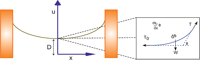\n",
"\n",
" **Figure 21.5** *Top:* A uniform string\n",
"suspended from its ends in a gravitational field assumes a catenary\n",
"shape. *Bottom:* A force diagram of a section of the catenary at its\n",
"lowest point. Because the ends of the string must support the entire\n",
"weight of the string, the tension now varies along the string.\n",
"\n",
"### 21.4.2 Derivation of Catenary Shape\n",
"\n",
"Consider a string of uniform density $\\rho$ acted upon by gravity. To avoid\n",
"confusion with our use of $y(x)$ to describe a disturbance on a string, we call\n",
"$u(x)$ the equilibrium shape of the string (Figure 21.5). The statics problem we\n",
"need to solve is to determine the shape $u(x)$ and the tension $T(x)$. The inset\n",
"in Figure 21.5 is a free-body diagram of the midpoint of the string and shows\n",
"that the weight $W$ of this section of arc length $s$ is balanced by the vertical\n",
"component of the tension $T$. The horizonal tension $T_0$ is balanced by the\n",
"horizontal component of $T$:\n",
"\n",
" $$\\begin{align}\n",
"\\tag*{21.35}\n",
"T(x)\\sin\\theta & = W = \\rho g s, \\quad T(x)\\cos\\theta = T_0,\\\\\n",
"\\Rightarrow \\quad \\tan\\theta & = {\\rho g s} /{T_0}. \\tag*{21.36}\\end{align}$$\n",
"\n",
"The trick is to convert (21.35) to a differential equation that we can solve. We\n",
"do that by replacing the slope $\\tan\\theta$ by the derivative $du/dx$, and\n",
"taking the derivative with respect to $x$:\n",
"\n",
"$$\\begin{align}\n",
"\\tag*{21.37}\n",
"\\frac{du}{dx} =\\frac{\\rho g} {T_0} s, \\quad \\Rightarrow\\quad\n",
"\\frac{d^2u} {dx^2} = \\frac {\\rho g} {T_0} \\frac{ds} {dx}.\\end{align}$$\n",
"\n",
"Yet because $ds = \\sqrt{dx^2+du^2}$, we have our differential equation\n",
"\n",
"$$\\begin{align}\n",
"\\tag*{21.38}\n",
"\\frac{d^2u} {dx^2} & = \\frac{1} {D} \\frac{\\sqrt{dx^2+du^2}} {dx}\n",
"= \\frac{1} {D} \\sqrt{1+ \\left( \\frac{du}{dx}\\right)^2},\\\\\n",
" D & = {T_0 / \\rho g},\\tag*{21.39}\\end{align}$$ \n",
" \n",
"where $D$ is a\n",
"combination of constants with the dimension of length. Equation (21.38) is the\n",
"equation for the *catenary* and has the solution \\[[Becker(54)](BiblioLinked.html#becker)\\] \n",
"\n",
"$$\\tag*{21.40}\n",
" u(x) = D \\cosh \\frac{x} {D}.$$\n",
"\n",
"Here we have chosen the $x$ axis to lie a distance $D$ below the bottom\n",
"of the catenary (Figure 21.5) so that $x=0$ is at the center of the\n",
"string where $y=D$ and $T=T_0$. Equation (21.37) tells us the arc length\n",
"$s= D du/dx$, so we can solve for $s(x)$ and for the tension $T(x)$ via\n",
"(21.35):\n",
"\n",
"$$\\tag*{21.41} s(x) = D \\sinh \\frac{x} {D},\\quad\\Rightarrow\\quad T(x) = T_0\n",
"\\frac{ds} {dx} = \\rho g u(x) = T_0 \\cosh\n",
"\\frac{x}{D}.$$\n",
"\n",
"It is this variation in tension that causes the wave velocity to change\n",
"for different positions on the string.\n",
"\n",
"### 21.4.3 Catenary and Frictional Wave Exercises\n",
"\n",
"[Movie of wave motion of a plucked catenary with friction.](http://science.oregonstate.edu/~rubin/Books/CPbook/eBook/Movies/CatFrictionAnimate.mp4)\n",
"\n",
"\n",
"\n",
"**Figure 21.6** The wave motion of a\n",
" plucked catenary with friction. (Courtesy of Juan Vanegas.)\n",
" \n",
"We have given you the program `EqStringAnimate.py` (Listing 21.1) that\n",
"solves the wave equation. Modify it to produce waves on a catenary\n",
"including friction for the assumed density and tension given by (21.32)\n",
"with $\\alpha\n",
"= 0.5$, $T_0=40$ N, and $\\rho_0=0.01$ kg/m. (The instructor’s site\n",
"contains the programs `CatFriction.py` and `CatString.py` that do this.)\n",
"\n",
"1. Look for some interesting cases and create surface plots of\n",
" the results.\n",
"\n",
"2. Describe in words how the waves dampen and how a wave’s velocity\n",
" appears to change.\n",
"\n",
"3. **Normal modes:** Search for normal-mode solutions of the\n",
" variable-tension wave equation, that is, solutions that vary as\n",
"\n",
" $$\\tag*{21.42}\n",
" u(x,t) = A \\cos(\\omega t)\\sin(\\gamma x).$$\n",
"\n",
" Try using this form to start your program and see if you can find\n",
" standing waves. Use large values for $\\omega$.\n",
"\n",
"4. When conducting physics demonstrations, we set up standing-wave\n",
" patterns by driving one end of the string periodically. Try doing\n",
" the same with your program; that is, build into your code the\n",
" condition that for all times\n",
"\n",
" $$\\tag*{21.43}\n",
" y(x=0,t) = A \\sin\\omega t.$$\n",
"\n",
" Try to vary $A$ and $\\omega$ until a normal mode (standing wave)\n",
" is obtained.\n",
"\n",
"5. (For the exponential density case.) If you were able to find\n",
" standing waves, then verify that this string acts like a\n",
" high-frequency filter, that is, that there is a frequency below\n",
" which no waves occur.\n",
"\n",
"6. For the catenary problem, plot your results showing *both* the\n",
" disturbance $u(x,t)$ about the catenary and the actual height\n",
" $y(x,t)$ above the horizontal for a plucked string\n",
" initial condition.\n",
"\n",
"7. Try the first two normal modes for a uniform string as the initial\n",
" conditions for the catenary. These should be close to, but not\n",
" exactly, normal modes.\n",
"\n",
"8. We derived the normal modes for a uniform string after assuming that\n",
" $ k(x) = {\\omega} /{c(x)}$ is a constant. For a catenary without too\n",
" much $x$ variation in the tension, we should be able to make the\n",
" approximation\n",
"\n",
" $$\\tag*{21.44}\n",
" c(x)^2 \\simeq \\frac{T(x)} {\\rho} = \\frac{T_0\\cosh\n",
" ({x}/{d})}{\\rho}.$$\n",
"\n",
" See if you get a better representation of the first two normal modes\n",
" if you include some $x$ dependence in $k$."
]
},
{
"cell_type": "markdown",
"metadata": {},
"source": [
"## 21.5 Vibrating Membrane (2-D Waves) \n",
"\n",
"**Problem:** An elastic membrane is stretched across the top of a square\n",
"box of sides $\\pi$ and attached securely. The tension per unit length in\n",
"the membrane is $T$. Initially the membrane is placed in the\n",
"asymmetrical shape,\n",
"\n",
"$$\\tag*{21.45} u(x,y,t=0) =\\sin 2x \\sin y, \\hspace{6ex} 0\\leq x \\leq \\pi,\n",
"\\quad 0\\leq y \\leq \\pi,$$\n",
"\n",
"where $u$ is the vertical displacement from equilibrium. Your\n",
"**problem** is to describe the motion of the membrane when it is\n",
"released from rest \\[[Kreyszig(98)](BiblioLinked.html#kreysig)\\].\n",
"\n",
"The description of wave motion on a membrane is basically the same as\n",
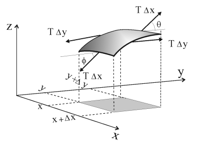
"that of 1-D waves on a string discussed in § 21.2, only now we have wave\n",
"propagation in two directions. Consider Figure 21.7 showing a square\n",
"section of the membrane under tension $T$. The membrane moves only\n",
"vertically in the $z$ direction, yet because the restoring force arising\n",
"from the tension in the membrane varies in both the $x$ and $y$\n",
"directions, there is wave motion along the surface of the membrane.\n",
"\n",
"\n",
"\n",
"**Figure 21.7** A small part of an oscillating membrane and the forces that act\n",
"on it.\n",
"\n",
"Although the tension is constant over the small area in Figure 21.7,\n",
"there will be a net vertical force on the segment if the angle of\n",
"incline of the membrane varies as we move through space. Accordingly,\n",
"the net force on the membrane in the $z$ direction as a result of the\n",
"change in $y$ is\n",
"\n",
"$$\\tag*{21.46}\n",
" \\sum F_z(x) \\ =\\ T\\Delta x \\sin\\theta - T \\Delta x \\sin \\phi,$$\n",
"\n",
"where $\\theta$ is the angle of incline at $y+\\Delta y$ and $\\phi$ the\n",
"angle at $y$. Yet if we assume that the displacements and the angles are\n",
"small, then we can make the approximations:\n",
"\n",
"$$\\begin{align}\n",
"\\tag*{21.47}\n",
" \\sin \\theta \\approx\\ \\tan \\theta &= \\frac{\\partial u}{ \\partial y}\\Bigr |_{y+\\Delta y},\\quad\n",
" \\sin \\phi \\approx\\ \\tan \\phi\n",
" = \\frac{\\partial u}{ \\partial y}\\Bigr |_{y} , \\\\\n",
" \\Rightarrow \\sum F_z(x_{fixed}) & = T\\Delta x \\Bigl (\n",
" \\frac{\\partial u}{ \\partial y}\\Bigr |_{y+\\Delta y}-\n",
" \\frac{\\partial u}{ \\partial y}\\Bigr |_{y} \\Bigr )\n",
"\\ \\approx\\ T\\Delta x \\frac{\\partial^2 u}{\\partial y^2} \\Delta y.\\tag*{21.48}\n",
" \\end{align}$$\n",
"\n",
"Similarly, the net force in the $z$ direction as a result of the\n",
"variation in $y$ is:\n",
"\n",
"$$\\tag*{21.49}\n",
" \\sum F_z (y_{fixed})\n",
" \\ =\\ T\\Delta y \\Bigl ( \\frac{\\partial u}{ \\partial x}\\Bigr |_{x+\\Delta x}-\n",
" \\frac{\\partial u}{ \\partial x}\\Bigr |_{x} \\Bigr )\n",
" \\ \\approx\\ T\\Delta y \\frac{\\partial^2 u}{\\partial x^2} \\Delta x.$$\n",
"\n",
"The membrane section has mass $\\rho\\Delta x\\Delta y$, where $\\rho$ is the\n",
"membrane’s mass per unit area. We now apply Newton’s second law to\n",
"determine the acceleration of the membrane section in the $z$ direction as a\n",
"result of the sum of the net forces arising from both the $x$ and $y$ variations:\n",
"\n",
"$$\\begin{align} \\tag*{21.50}\n",
"\\rho\\Delta x\\Delta y \\frac{\\partial^2 u}{\\partial t^2} & = \\Delta x \\frac{\\partial^2 u}{\\partial y^2}\n",
"\\Delta y+ T\\Delta y \\frac{\\partial^2 u}{\\partial x^2} \\Delta x, \\\\\n",
"\\Rightarrow\\hspace{6ex} \\frac{1}{ c^2} \\frac{\\partial ^2u}{ \\partial t^2} \\ & =\\\n",
" \\frac {\\partial ^2 u }{ \\partial x^2} + \\frac{\\partial ^2 u }{ \\partial y^2},\n",
" \\hspace{6ex} c \\ =\\ \\sqrt{ {T}/{\\rho}}.\\tag*{21.51}\\end{align}$$\n",
"\n",
"This is the 2-D version of the wave equation (21.4) that we studied\n",
"previously in one dimension. Here $c$, the propagation velocity, is\n",
"still the square root of tension over density, only now it is tension\n",
"per unit length and mass per unit area."
]
},
{
"cell_type": "markdown",
"metadata": {},
"source": [
"## 21.6 Analytical Solution \n",
"\n",
"The analytic or numerical solution of the partial differential equation\n",
"(21.51) requires us to know both the boundary conditions and the initial\n",
"conditions. The boundary conditions hold for all times and were given\n",
"when we were told that the membrane is attached securely to a square box\n",
"of side $\\pi$:\n",
"\n",
"$$\\begin{align}\\tag*{21.52}\n",
" u(x=0,y,t) &\\ =\\ u(x=\\pi, y,t)\\ =\\ 0, \\\\\n",
" u(x,y=0,t) &\\ =\\ u(x, y=\\pi ,t)\\ =\\ 0.\\tag*{21.53}\n",
" \\end{align}$$\n",
"\n",
"As required for a second order equation, the initial conditions has two\n",
"parts, the shape of the membrane at time $t=0$, and the velocity of each\n",
"point of the membrane. The initial configuration is\n",
"\n",
"$$\\tag*{21.54}\n",
" u(x,y,t=0) \\ =\\ \\sin 2x \\sin y, \\hspace{6ex} 0\\leq x \\leq \\pi,\n",
" 0\\leq y \\leq \\pi.$$\n",
"\n",
"Second, we are told that the membrane is released from rest, which\n",
"means:\n",
"\n",
"$$\\tag*{21.55}\n",
"\\frac{\\partial u }{ \\partial t}\\Bigl |_{t=0} =0,$$\n",
"\n",
"where we write partial derivative because there are also spatial\n",
"variations.\n",
"\n",
"The analytic solution is based on the guess that because the wave\n",
"equation (21.51) has separate derivatives with respect to each\n",
"coordinate and time, the full solution $u(x,y,t)$ is the product of\n",
"separate functions of $x$, $y$ and $t$:\n",
"\n",
"$$\\tag*{21.56}\n",
" u(x,y,t)= X(x) Y(y) T(t).$$\n",
"\n",
"After substituting this into (21.51) and dividing by $X(x)Y(y) T(t)$, we\n",
"obtain:\n",
"\n",
"$$\\tag*{21.57}\n",
"\\frac{1}{ c^2} \\frac{1}{ T(t)} \\frac{d^2T(t)}{ dt^2}\\ \\ =\\ \\ \\frac{1}{\n",
"X(x)} \\frac{d^2 X(x)}{ dx^2} + \\frac{1}{ Y(y)} \\frac{d^2 Y(y)}{\n",
"dy^2}.$$\n",
"\n",
"The only way that the LHS of (21.57) can be true for all time while the\n",
"RHS is also true for all coordinates, is if both sides are constant:\n",
"\n",
"$$\\begin{align}\\tag*{21.58}\n",
" \\frac{1}{ c^2} \\frac{1}{ T(t)} \\frac{d^2T(t)}{ dt^2} \n",
" &= -\\xi^2 = \\frac {1} { X(x)} \\frac{d^2 X(x)}{ dx^2} + \\frac{1}{ Y(y)}\n",
" \\frac {d^2 Y(y)}{ dy^2} , \\\\\n",
" \\Rightarrow \\frac{1}{ X(x)} \\frac{d^2X(x)}{ dx^2} &= -k^2,\\tag*{21.59}\\\\\n",
"\\frac{1}{ Y(y)} \\frac {d^2Y(y)}{ dy^2} &= -q^2, \\qquad\n",
"(q^2 = \\xi^2 -k^2).\\tag*{21.60}\n",
" \\end{align}$$\n",
"\n",
"In (21.59) and (21.60) we have included the further deduction that\n",
"because each term on the RHS of (21.58) depends on either $x$ or $y$,\n",
"then the only way for their sum to be constant is if each term is a\n",
"constant, in this case $-k^2$. The solutions of these equations are\n",
"standing waves in the $x$ and $y$ directions, which of course are all\n",
"sinusoidal function,\n",
"\n",
"$$\\begin{align}\n",
"\\tag*{21.61}\n",
" X(x) &\\ =\\ A \\sin kx + B \\cos kx, \\\\\n",
" Y(y) &\\ =\\ C \\sin qy + D \\cos qy, \\tag*{21.62} \\\\\n",
" T(t)&\\ =\\ E \\sin c\\xi t + F \\cos c\\xi t.\\tag*{21.63}\n",
" \\end{align}$$\n",
"\n",
"We now apply the boundary conditions:\n",
"\n",
"$$\\begin{align}\n",
" u(x=0,y,t) &= u(x=\\pi,y,z)=0 \\Rightarrow B=0, k =1,2,\\cdots, \\\\\n",
" u(x,y=0,t) & = u(x, y=\\pi ,t)=0\n",
" \\Rightarrow D=0, q =1,2,\\cdots, \\\\\n",
" \\Rightarrow X(x)& \\ = A\\sin kx, Y(y)= C\\sin qy.\\tag*{21.64}\n",
" \\end{align}$$\n",
"\n",
"The fixed values for the eigenvalues $m$ and $n$ describing the modes\n",
"for the $x$ and $y$ standing waves are equivalent to fixed values for\n",
"the constants $q^2$ and $k^2$. Yet because $q^2 + k^2 = \\xi^2$, we must\n",
"also have a fixed value for $\\xi^2$:\n",
"\n",
"\\begin{equation}\\tag*{21.65}\n",
" \\xi^2 = q^2 + k^2 \\hspace{6ex} \\Rightarrow \\hspace{6ex}\n",
" \\xi_{kq}=\\pi\\sqrt{k^2 +q^2}.\n",
" \\end{equation}\n",
"\n",
"The full space-time solution now takes the form\n",
"\n",
"\\begin{equation}\\tag*{21.66}\n",
" u_{kq}= \\left[G_{kq}\\cos c\\xi t +H_{kq} \\sin c\\xi t\\right] \\sin k x \\sin\n",
" q y,\n",
" \\end{equation}\n",
"\n",
"where $k$ and $q$ are integers. Because the wave equation is linear\n",
"in $u$, its most general solution is a linear combination of the\n",
"eigenmodes (21.66):\n",
"\n",
"\\begin{equation}\\tag*{21.67}\n",
" u(x,y,t)=\\sum_{k=1}^\\infty \\sum_{q=1}^\\infty \\left[G_{kq}\\cos c\\xi t\n",
" +H_{kq} \\sin c\\xi t \\right] \\sin k x \\sin q y.\n",
" \\end{equation}\n",
" \n",
"While an infinite series is not a good algorithm, the\n",
"initial and boundary conditions means that only the $k=2$,\n",
"$q=1$ term contributes, and we have a closed form solution:\n",
"\n",
"\\begin{equation}\\tag*{21.68}\n",
"u(x,y,t)= \\cos c\\sqrt{5} \\ \\sin 2x\\ \\sin y,\n",
" \\end{equation}\n",
"\n",
"where $c$ is the wave velocity. You should verify that initial and\n",
"boundary conditions are indeed satisfied.\n",
"\n",
"\n",
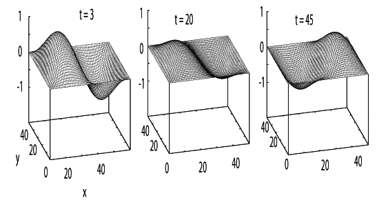
"\n",
"**Figure 21.8 ** The standing wave pattern on a square box top at three\n",
"different times.\n",
"\n",
"[**Listing 21.1 Waves2D.py**](http://www.science.oregonstate.edu/~rubin/Books/CPbook/Codes/PythonCodes/Waves2D.py) solves the wave equation numerically for a vibrating membrane."
]
},
{
"cell_type": "markdown",
"metadata": {
"collapsed": true
},
"source": [
"## 21.7 Numerical Solution for 2-D Waves\n",
"\n",
"The development of an algorithm for the solution of the 2-D wave\n",
"equation (21.51) follows that of the 1-D equation in\n",
"\\S~21.2.2. We start by expressing the second derivatives in\n",
"terms of central differences:\n",
"\n",
"$$\\begin{align}\\tag*{21.69}\n",
"\\frac{\\partial^2 u(x,y,t)}{ \\partial t^2} &\\ =\\ \\frac{u(x,y,t+\\Delta t) +\n",
"u(x,y,t-\\Delta t) -2u(x,y,t) }{ (\\Delta t)^2}, \\\\\n",
"\\frac{\\partial^2 u(x,y,t)}{ \\partial x^2} &\\ =\\\n",
"\\frac{u(x+\\Delta x,y,t) + u(x-\\Delta x,y,t) -2u(x,y,t) }{ (\\Delta x)^2}, \\tag*{21.70}\\\\\n",
"\\frac{\\partial^2 u(x,y,t)}{ \\partial y^2} &\\ =\\ \\frac{u(x,y+\\Delta y,t) +\n",
"u(x,y-\\Delta y,t) -2u(x,y,t) }{ (\\Delta y)^2}.\\tag*{21.71}\\end{align}$$\n",
"\n",
"After discretizing the variables, $u(x= i\\Delta, y=i\\Delta\n",
"y,t=k\\Delta t) \\equiv u^k_{i,j}$, we obtain our time-stepping algorithm\n",
"by solving for the future solution in terms of the present and past\n",
"ones:\n",
"\n",
"$$\\tag*{21.72}\n",
"\\boxed{u^{k+1}_{i,j} = 2u^k_{i,j}-u^{k-1}_{i,j} \\frac{c^2}{c'^2} \\Bigl [u^{k}_{i+1,j}\n",
" + u^{k}_{i-1,j}\n",
" -4u^k_{i,j}\n",
"+ {u^{k}_{i,j+1} + u^{k}_{i,j-1} } \\Bigr ],}$$\n",
"\n",
"where as before $c' = \\Delta x/ \\Delta t$. Whereas the present ($k$)\n",
"and past ($k-1$) solutions are known after the first step, to initiate\n",
"the algorithm we need to know the solution at $t=-\\Delta t$, that is,\n",
"before the initial time. To find that, we use the fact that the membrane\n",
"is released from rest:\n",
"\n",
"$$\\tag*{21.73} 0 = \\frac{\\partial u (t=0)}{\\partial t} \\approx\n",
"\\frac{u^1_{i,j}-u^{-1}_{i,j}} { 2\\Delta t}, \\hspace{6ex}\n",
"\\Rightarrow\\hspace{6ex} u^{-1}_{i,j} =u^1_{i,j}.$$\n",
"\n",
"After substitution into (21.72) and solving for $u^1$, we obtain the\n",
"algorithm for the first step:\n",
"\n",
"$$\\tag*{21.74} u^1_{i,j} = u^0_{i,j}+ \\frac{c^2}{ 2 c'^2} \\Bigl [u^{0}_{i+1,j}\n",
" + u^{0}_{i-1,j}\n",
" -4u^0_{i,j}\n",
"+ {u^{0}_{i,j+1} + u^{0}_{i,j-1} } \\Bigr ].$$\n",
"\n",
"Because the displacement $u^0_{i,j}$ is known at time $t=0$ ($k=0$), we\n",
"compute the solution for the first time step with (21.74) and for\n",
"subsequent steps with (21.72).\n",
"\n",
"The program `Wave2D.py` in Listing 21.2 solves the 2-D wave equation\n",
"using the time-stepping (leapfrog) algorithm. The program\n",
"`Waves2Danal.py` computes the analytic solution. The shape of the\n",
"membrane at three different times are shown in Figure 21.8."
]
},
{
"cell_type": "code",
"execution_count": null,
"metadata": {
"collapsed": false
},
"outputs": [],
"source": [
"### VibratingMembrane.py, Notebook Version\n",
"\n",
"import numpy as np\n",
"import matplotlib.pyplot as plt\n",
"import mpl_toolkits.mplot3d.axes3d \n",
"\n",
"t=0 # initial time\n",
"den=390.0 #density kg/m2\n",
"ten=180.0 # tension N/m2\n",
"c=np.sqrt(ten/den) # propagation velocity\n",
"s5=np.sqrt(5)\n",
"N=32\n",
"t=0\n",
"\n",
"def membrane(t,X,Y): # analytic solution vibrating membrane\n",
" return np.cos(c * s5* t) * np.sin( 2* X)*np.sin(Y) \n",
"\n",
"plt.ion() # interactive on\n",
"fig=plt.figure()\n",
"ax = fig.add_subplot(111, projection='3d')\n",
"xs=np.linspace(0, np.pi,32) # 0 to pi increm: pi/32\n",
"ys=np.linspace(0, np.pi,32) # same\n",
"X, Y = np.meshgrid(xs,ys) # define x,grid\n",
"Z = membrane(0, X, Y) # initial condition t=0\n",
"wframe = None\n",
"ax.set_xlabel('X') # name x axis\n",
"ax.set_ylabel('Y')\n",
"ax.set_title('Vibrating membrane')\n",
"for t in np.linspace(0,50,200): #total time 10 divided by 40\n",
" oldcol=wframe # previous frame\n",
" Z=membrane(t,X,Y) # membrane at t !=0\n",
" wframe=ax.plot_wireframe(X,Y,Z)# plot the wireframe\n",
" # Remove old frame before drawing\n",
" if oldcol is not None:\n",
" ax.collections.remove(oldcol)\n",
"\n",
" plt.draw() #plot new frame\n",
"print(\"finished\")"
]
},
{
"cell_type": "code",
"execution_count": null,
"metadata": {
"collapsed": true
},
"outputs": [],
"source": []
}
],
"metadata": {
"kernelspec": {
"display_name": "Python 2",
"language": "python",
"name": "python2"
},
"language_info": {
"codemirror_mode": {
"name": "ipython",
"version": 2
},
"file_extension": ".py",
"mimetype": "text/x-python",
"name": "python",
"nbconvert_exporter": "python",
"pygments_lexer": "ipython2",
"version": "2.7.11"
}
},
"nbformat": 4,
"nbformat_minor": 0
}